Orthogonal Forward Regression based on Directly Maximizing
Model Generalization Capability
S. Chen
Ýand X. Hong
ÞÝ
Department of Electronics and Computer Science
University of Southampton, Southampton SO17 1BJ, UK
Þ
Department of Cybernetics
University of Reading, Reading, RG6 6AY, UK
Abstract
The paper introduces a construction algorithm for sparse kernel modelling using the leave-one-out test score also known as the PRESS (Predicted REsidual Sums of Squares) statistic. An efficient subset model selection procedure is developed in the orthogonal forward regression framework by incrementally maximizing the model generalization ca-pability to construct sparse models with good generaliza-tion properties. The proposed algorithm achieves a fully automated model construction without resort to any other validation data set for costly model evaluation.
Index Terms — orthogonal forward regression, structure
identification, cross validation, generalization.
1 Introduction
The least squares (LS) principle has been fundamental to data modelling and the training mean square error (MSE) has always played a central role in model structure con-struction and parameter estimation. It is well known that the model based on the pure LS estimate tend to be unsatisfac-tory for an ill conditioned design matrix, and may over-fit the noise in training data to produce an oversized ill-posed model with high parameter estimate variances. To produce a model with good generalization capabilities, model selec-tion criteria such as the Akaike informaselec-tion criterion (AIC) [1], local regularization and optimal experimental design [2]–[4] incorporate some sorts of model structure regular-ization with the basic training MSE criterion. In forward regression setting [5], which is a practical way of construct-ing a kernel model from a large data set, local regularization and optimal experimental design criteria are known to offer better solutions [2]–[4], compared with the AIC.
In order to achieve a model structure with improved model generalization, it is natural that a model generalization ca-pability cost function should be used in the overall model searching process, rather than only being applied as a mea-sure of model complexity. Because the evaluation of the model generalization capability is directly based on the
con-cept of cross validation [6], it is highly desirable to develop model selective criteria based on the concept of cross vali-dation that can distinguish model generalization capability during the model construction process. A fundamental con-cept in cross validation is that of delete-1 cross validation in statistics, and the associated concept of the leave-one-out test score also known as the PRESS (Predicted REsidual Sums of Squares) statistic [7]–[9]. The leave-one-out test score is a measure of model generalization capability. Tra-ditional model structure determination based on the leave-one-out test score or PRESS statistic is however inherently inefficient and computationally prohibitive.
The paper introduces an efficient automatic model con-struction algorithm that directly optimizes model general-ization capability. The computational efficiency is achieved through incrementally minimizing the leave-one-out test score in an orthogonal forward regression framework, which minimizes the effort in the computation of the PRESS statistic. Further significant reduction in computation arises owing to a forward recursive formula to compute PRESS er-rors. In the proposed algorithm, the PRESS statistic, which is a measure of model generalization capability, is applied directly in the orthogonal forward regression model struc-ture construction process as a cost function in order to op-timize the model generalization capability. The proposed algorithm achieves a fully automatic model selection pro-cedure without resorting to another validation data set for model assessment. Two examples are included to demon-strate the effectiveness of the approach.
2 Kernel modelling
Consider a general discrete stochastic nonlinear system rep-resented by [10]:
(1)
whereand are the system input and output
vari-ables, respectively, and
are positive integers
observation noise is uncorrelated with zero mean and
variance ,
denotes the system input vector, is a priori
un-known system mapping, and is an unknown parameter vector associated with the model structure. The system model (1) is to be identified from an-sample system
ob-servational data set
.
Consider the modelling of the unknown dynamical process (1) by using a linear-in-the-parameters model of the form:
(2)
where is the number of candidate regressors,
,
are the model weights and
the model parameter vector. The model (2) for can be written in the matrix form as
(3)
where
is the desired output
vec-tor,
is the residual vector, and
is the regression matrix with
, . An orthogonal
de-composition ofcan be expressed as
(4)
where
is anupper triangular matrix with
unity diagonal elements andis anmatrix having
orthogonal columns that satisfies
(5)
with
,
. The model (3) can
alterna-tively be expressed as
(6)
in which
is the orthogonal weight vector. Knowing, the original model weight vector can be
cal-culated from . The space spanned by the original
model bases
,, is identical to
that spanned by the orthogonal bases
, ,
and the model (2) is equivalently expressed by
(7)
where
.
3 Orthogonal forward regression using PRESS statistic
Consider the model selection problem for modelling (1) by a set of models, indexed by , that are
based on a variety of model structures. Denote these models
as
if they are identified using all thedata points
in . To optimize the model generalization capability, the
model selection criteria are often based on cross-validation [6], and one commonly used version of cross validation is called delete-1 cross validation [8],[9]. The idea is that, for every model, each data point in the training data set is
sequentially set aside in turn, a model is estimated using the remaining data points, and the prediction error is
de-rived using only the data point that was removed from the estimation data set. Specifically, let
be the resulting data set by removing the-th data point from
, and
de-note the-th model estimated using
as
and the related predicted model residual atas:
(8)
The leave-one-out test score or the mean square PRESS er-ror [8],[9] for the-th model
is obtained by
averaging all these prediction errors:
(9)
To select the best model from thecandidates
,
, the same modelling process is applied to all
themodels, and the predictor with the minimum PRESS
statistic is selected, i.e. the -th model is selected if
(10)
For linear-in-the-parameters models, the PRESS statistic can be generated without actually sequentially splitting the training data set and repeatedly estimating the associated models [8]. Consider that an-term model
is
identified using based on the model form of (2). The
PRESS errors
can be calculated using [8],[9]:
(11)
where
. Obviously,
choos-ing the best subset model that minimizes the PRESS statis-tic quickly becomes computationally prohibitive even for a modest-term model set. Moreover, the PRESS error
(11) itself is computational expensive because the matrix inversion involved. However, if we choose only to incre-mentally minimize the PRESS statistic in an orthogonal for-ward regression manner with an efficient computation of the PRESS error, the model selection procedure based on the PRESS statistic becomes computationally affordable.
It can readily be shown that the PRESS error
for the-term orthogonal weight model (7) is given by:
assuming that regularization is applied with a regularization
parameter, where is an
diagonal matrix and
(13)
Consider the orthogonal forward regression, in which a sub-set model of theregressors () is selected from the
full model set consisting of the initial regressors given
by (7). The PRESS errors (12) and (13) can be written, by replacingwith a variable model size, as
(14)
where
(15)
and
is the model residual associated with the
sub-set model structure consisting of theselected regressors.
can be written as a recursive formula, given by
(16)
As is in the conventional orthogonal LS algorithm [5], a Gram-Schmidt procedure is used to construct the orthogo-nal basis
in a forward regression manner. At each
re-gression step, the PRESS statistic can be computed with:
(17)
and this is used as the regressor selective criterion for the model construction which minimizes this mean square PRESS error. Note that the function
is concave
ver-sus , and there exists an “optimal” model size such
that for
decreases as
increases, while for
increases as
increases [11]. This property,
i.e.
changes the sign at certain model size , can be applied to construct the automatic algorithm.
The proposed algorithm selects significant regressors that minimizes the PRESS statistic, with a growing model struc-ture until at a desired model size , where the
contribution of the th regressor in model
approxima-tion becomes insignificant. Thus the algorithm terminates at
·½
, where the model is optimized based on the
minimization of the PRESS statistics at
. Note that
nei-ther a separate criterion to terminate the selection procedure nor any iteration of the procedure is needed. The proposed algorithm based on the standard Gram-Schmidt procedure is summarized in Appendix, in which the orthogonal ba-sis is constructed in a forward regression manner. In
this algorithm a small fixed positive regularization parame-ter, e.g.
, is used to improve parameter estimation variance. Note that the algorithm selects only those model terms which satisfy . Thus any numerical
ill-conditioning problem is automatically avoided.
4 Numerical examples
Two examples were used to demonstrate the effectiveness of the proposed model construction algorithm.
Example 1. Consider using a radial basis function (RBF)
network to approximate an unknown scalar function
(18)
Four hundred training data were generated from
, where the inputwas uniformly distributed in
and the noisewas Gaussian with zero mean and standard
deviation 0.2. The first two hundred samples were used for training and the last two hundred data points for possible model validation. The Gaussian basis function
(19)
was used, with a kernel width . All the two
hun-dred training data points were used as the candidate RBF center set for . Two hundred noise-free data
with
equally spacedin were also generated as an
[image:3.612.100.284.413.472.2]ad-ditional testing data set for evaluating model performance. The regularization parameter was fixed to.
Fig. 1 depicts the evolution of the training MSE and PRESS statistic inscale during the orthogonal forward
regres-sion with a typical set of noisy training data using the pro-posed algorithm. It can be seen from Fig. 1 that the PRESS statistic continuously decreased until
, and the algorithm terminated with a 7-term
model. Fig. 2 shows the noisy training points and the un-derlying function together with the mapping generated
0.1
0 1 2 3 4 5 6 7 8 9
Model MSE and PRESS statistic
Model size PRESS
MSE
[image:3.612.332.535.554.694.2]
[image:4.612.333.530.41.340.2]
Figure 2:Simple scalar function modelling problem: a typical set of noisy training data (dots), underlying function
(thin curve), model mapping (thick curve), and
selected RBF centers (circles). The 7-term model was identified without the help of a validation set.
using this 7-term model identified. Table 1 summarizes the modelling accuracy (mean standard deviation) averaged
over ten sets of different data realizations. It can be seen that the proposed algorithm was able to produce very sparse models with excellent generalization performance, without the need to use additional validation set for model evalua-tion during the model construcevalua-tion process.
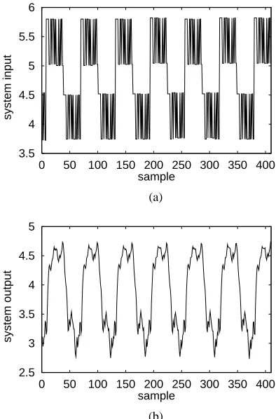
Example 2. This example constructed a model
represent-ing the relationship between the fuel rack position (input
) and the engine speed (output ) for a Leyland TL11
turbocharged, direct injection diesel engine operated at low engine speed. Detailed system description and experimental setup can be found in [12]. The data set, depicted in Fig. 3, contained 410 samples. The first 210 data points were used in training and the last 200 points in possible model valida-tion. A RBF model with the input vector
(20)
and the Gaussian basis function of variance was
used to model the data. All the 210 training data points were used as the candidate RBF centre set and the regularisation parameter was fixed to
[image:4.612.58.285.42.173.2]
.
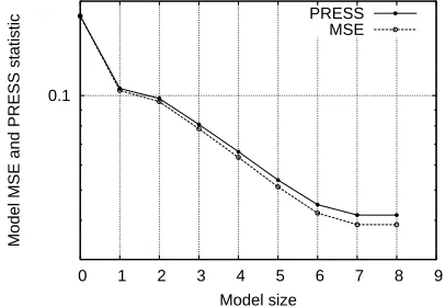
Fig. 4 shows the evolution of the training MSE and PRESS statistic during the forward regression procedure, where it can be seen that the PRESS statistic continuously decreased until
. The
algo-rithm thus automatically terminated with a 23-term model.
Table 1:Modelling accuracy (meanstandard deviation) over
ten sets of different data realizations for simple scalar function modelling.
model terms
MSE over training set
PRESS statistic
MSE over noisy test set
MSE over noise-free test set
3.5 4 4.5 5 5.5 6
0 50 100 150 200 250 300 350 400
system input
sample
(a)
2.5 3 3.5 4 4.5 5
0 50 100 150 200 250 300 350 400
system output
sample
(b)
Figure 3:Engine data set (a) inputand (b) output .
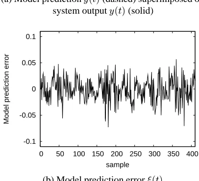
The modelling accuracy is summarized in Table 2. The constructed RBF model
was used to generate the
model prediction according to
(21)
with the input vector given by (20). Fig. 5 depicts
the model prediction and the prediction error
for the 23-term model constructed. Again, it is
seen that the proposed algorithm was able to produce very sparse models with excellent generalization performance, without the need to use additional validation set for model evaluation during the model construction process.
1e-4 1e-3 1e-2 1e-1 1 10
0 5 10 15 20 25
Model MSE and PRESS statistic
Model size PRESS
MSE
[image:4.612.343.536.553.694.2]Table 2:Modelling accuracy for engine data set modelling.
model terms 23
MSE over training set 0.000449 PRESS statistic 0.000548 MSE over test set 0.000487
5 Conclusions
This paper has introduced an automatic model construc-tion algorithm for linear-in-the-parameters nonlinear mod-els based directly on maximizing model generalization ca-pability. The leave-one-out test score or PRESS statistic in the framework of regularized orthogonal least squares has been derived and, in particular, an efficient recursive com-putation formula for PRESS errors has been developed. The proposed algorithm based on orthogonal forward regression combines parameter regularization technique in orthogonal weight space and the PRESS statistic to optimize model structure in order to achieve improved generalization capa-bility, without resorting to another validation data set for model assessment.
Appendix: Combined PRESS statistic and regularised orthogonal least squares for subset model selection
1. Initialization: initialize , and
for . For,
com-pute Find and select ½ ½ with ½ and for 2.5 3 3.5 4 4.5 5
0 50 100 150 200 250 300 350 400
System output/Model prediction
sample
(a) Model prediction (dashed) superimposed on
system output (solid)
-0.1 -0.05 0 0.05 0.1
0 50 100 150 200 250 300 350 400
Model prediction error
sample
[image:5.612.332.535.198.383.2](b) Model prediction error
Figure 5:Modelling performance for engine data set modelling problem. The 23-term model was constructed without the help of a validation set.
for
2. At theth step where , for and
Find
and select
with
and
for
for
3. The selection procedure is terminated with an
-term model at the step, when
.
Otherwise, set, and go to step 2.
References
[1] Akaike, H., 1974, “A new look at the statistical model identification,” IEEE Trans. Automatic Control, Vol.AC-19, pp.716–723.
[2] Chen, S., 2002, “Locally regularised orthogonal least squares algorithm for the construction of sparse kernel re-gression models,” in Proc. 6th Int. Conf. Signal Processing (Beijing, China), Aug.26-30, 2002, pp.1229–1232.
[3] Chen, S., Hong, X., and Harris, C.J., 2002, “Sparse data modelling using combined locally regularized orthog-onal least squares and D-optimality design,” in: Proc.
Com-bined Annual Conf. Institute of Automation, the Chinese Academy of Sciences, and Annual Conf. Chinese Automa-tion and Computer Science Society in U.K. (Beijing, China),
Sept.20-21, 2002, pp.112-117.
[4] Chen, S., Hong, X., and Harris, C.J., 2003, “Sparse kernel regression modelling using combined locally regular-ized orthogonal least squares and D-optimality experimen-tal design,” IEEE Trans. Automatic Control, to appear, June 2003.
[5] Chen, S., Billings, S.A., and Luo, W., 1989, “Orthog-onal least squares methods and their applications to non-linear system identification,” Int. J. Control, Vol.50, No.5, pp.1873–1896.
[6] Stone, M., 1974, “Cross validatory choice and assess-ment of statistical predictions,” J. R. Statist. Soc. Ser. B., Vol.36, pp.117–147.
[7] Breiman, L., 1996, “Stacked regression,” Machine
Learning, Vol.5, pp.49–64.
[8] Myers, R.H., 1990, Classical and Modern Regression
with Applications, 2nd Edition, Boston: PWS-KENT.
[9] Hansen, L.K., and Larsen, J., 1996, “Linear unlearn-ing for cross-validation,” Advances in Computational
Math-ematics, Vol.5, pp.269–280.
[10] Chen, S., and Billings, S.A., 1989, “Representation of non-linear systems: the NARMAX model,” Int. J.
Con-trol, Vol.49, No.3, pp.1013–1032.
[11] Hong, X., Sharkey, P.M., and Warwick, K., 2003, “Automatic nonlinear predictive model construction algo-rithm using forward regression and the PRESS statistic,”
IEE Proc. Control Theory and Applications, to appear.
[12] Billings, S.A., Chen, S., and Backhouse, R.J., 1989, “The identification of linear and non-linear models of a tur-bocharged automotive diesel engine,” Mechanical Systems