Longer Data, Less “CHEER”—Case Study of Yen Dollar Exchange Rate

(1)

ISSN Online: 2152-7261 ISSN Print: 2152-7245

DOI: 10.4236/me.2019.109129 Sep. 12, 2019 2051 Modern Economy

Longer Data, Less “CHEER”—Case Study of

Yen-Dollar Exchange Rate

Yan Zhao

1

_{, Shen Guo}

2

_{, Zhiqiang Ye}

1

1_{School of Business, East China University of Science and Technology, Shanghai, China} 2_{China Academy of Public Finance and Public Policy, CUFE, Beijing, China}

Abstract

This paper compares CHEER approach in both short-run (since 1973) and long-run (since 1870) with the yen-dollar exchange rate. The most important result is that CHEER is valid only in the period when the international capital market is developed enough. Historical data will render the interest rate pari-ty insignificant and thus CHEER will fail. Also, the paper demonstrates that when either PPP or UIP fails, modification of the cointegration variables im-proves the power of the CHEER test.

Keywords

PPP, UIP, CHEER, Exchange Rate

1. Introduction

The question of exchange rate determination has been the center of research in international economics and finance. In the literature, purchasing power parity (PPP), which was put forth by [1], probably is the first theory to measure the equilibrium exchange rate level. Empirical tests of PPP have been typically based on the investigation of the time series property of the real exchange rate, which can be seen as the residuals from PPP. These test results indicate that PPP may not hold: the failure of PPP in the short run is common. Even in the long run, the validity of PPP is mixed.

The failure of PPP caused many people to raise doubt on the PPP as the model of equilibrium exchange rate. With the great expansion of world financial mar-kets in the past thirty years, some researchers argue that the price levels are not sufficient to capture all the factors causing fluctuations of the exchange rate without taking the world financial markets into account. In terms of balance of

How to cite this paper: Zhao, Y., Guo, S. and Ye, Z.Q. (2019) Longer Data, Less “CHEER”—Case Study of Yen-Dollar Exchange Rate. Modern Economy, 10, 2051-2062.

https://doi.org/10.4236/me.2019.109129 Received: August 9, 2019

Accepted: September 9, 2019 Published: September 12, 2019

http://creativecommons.org/licenses/by/4.0/

(2)

DOI: 10.4236/me.2019.109129 2052 Modern Economy payments, PPP only represents the current account, while the capital account is by and large ignored. For this reason, the exchange rate deviation from PPP is not surprising because of the existence of non-zero interest rate differentials. Accordingly, a model that covers both the purchasing power parity and unco-vered interest parity (UIP) is more appropriate to forecast the equilibrium ex-change rate. This methodology, therefore, is called the capital enhanced equili-brium exchange rate (CHEER) approach by [2].

The CHEER approach was first proposed by [3] and then developed by [4]. Since then, the CHEER approach has become popular in the study of exchange rates. Extensively studied, the conclusion for CHEER is still mixed: some re-searchers find supportive evidence while others cannot.1

Considering the different exchange rates, dissimilar empirical methods and varying data span in CHEER tests, mixed results may not be unusual. Still, it is important to summarize the key characteristics of the current research. Careful review of these papers raises at least two questions. The first question is why the cointegration relationship is often investigated between prices, interest rates and the contemporaneous, not the expected future exchange rate? Substituting the current exchange rate for the future rate is not in consistency with the CHEER approach because UIP hypothesis describes the relationship between interest rates and expected future exchange rate, not the current rate. Therefore, literally speaking, PPP and UIP are not combined correctly in the papers where the con-temporaneous exchange rate is put to test.

IF PPP and UIP are the underlying theoretical framework for CHEER, then we have the second question: why PPP and UIP are not explicitly tested before checking CHEER? Or, equivalently, can the non-rejection of no cointegration be ascribed to the failure of PPP or UIP? This paper shows that either a failure of PPP or UIP does result in non-rejection of no-cointegration. The reason is that the linear sum of error terms in PPP and UIP will not be stationary if exactly one of them fails to hold.2_{In this case, it is impossible to find evidence supporting}

the CHEER approach. Modification of the variables under study, however, may increase the possibility of finding cointegration. Thus, an appropriate step in the investigation of whether PPP and UIP hold is essential to improve the power of cointegration analysis.

This paper aims at demonstrating that ignorance of the two above mentioned questions may be the reasons of mixed evidence for CHEER using the Yen/Dollar exchange rate. For the first question, perfect foresight is assumed to circumvent the lack of expectation in UIP testing. The result reveals that this simple modification is not trivial: cointegration among prices, interest rates and the exchange rate would not exist without adding expectations.

1_{For positive results, see}_[5]_,_[6]_,_[7]_{, etc. For the negative results, see}_[8]_,_[9]_,_[10]_[11]_{, and}_[12]_{, etc.} 2_{Here it is important to note that when both PPP and UIP fail, it becomes possible to find evidence}

(3)

DOI: 10.4236/me.2019.109129 2053 Modern Economy For the second question, this paper explicitly distinguishes short-run and long-run analysis. The short-run analysis consists of monthly data from 1973, while the long-run investigation covers annual data from the year 1870. This different treatment according to data span proves essential, yet in a very unex-pected way: although supportive evidence for CHEER is found in the short-run, it does not exist in the long-run. The econometric analysis reveals that this is because the relative interest rates become exogenous in the long run and it does not belong to the exchange rate determination system. The puzzling result can be explained from the development of international capital markets. The short-run analysis covers recent data when capital market becomes as important as the goods market. Most of the time in the long-run, in contrast, does not see well developed international capital market. Because the essence of CHEER ap-proach is to determine the exchange rate through both trade and finance mar-kets, it is not a surprise to see CHEER fail in the period when one market is not well developed.

The remainder of this paper is structured as follows. Sections 2 and 3 analyze the short-run and long-run, respectively. Section 4 summarizes this paper.

2. Short-Run Analysis

2.1. PPP and UIP

Let Pt and Pt∗ denote the price levels for the home and foreign country

re-spectively, and St represents the nominal exchange rate (foreign price of

do-mestic currency). PPP can be expressed as P S Pt = t t∗. By changing to lower-case

letters to denote the natural logs, it can be rewritten as:

.

t t t

s ₌p p₋ ∗ ₍₁₎ Traditionally, Equation (1) is referred as the absolute PPP and the relative PPP is its first order difference:

.

t t t

s p p∗

∆ = ∆ − ∆ ₍₂₎

Tests for PPP refers to the investigation of time series properties of the real exchange rate qt.

.

t t t t

q _{= −}s p ₊p∗ ₍₃₎ Uncovered Interest Parity (UIP) states that one unit of currency should have the same return whether invested in the domestic or the foreign markets at equi-librium. Let It and It∗ denote the domestic and foreign interest rates,

respec-tively, and E St

(

t+1

)

represents the expectation of nominal exchange rate at

pe-riod t+1, then UIP can be written as:

(

)

( )

1

1 1 t t ,

t t

t

E S

I I

S + ∗

+ = + ₍₄₎

or

( )

1 ,

t t t t t

E s s i i∗

(4)

DOI: 10.4236/me.2019.109129 2054 Modern Economy where st =log

( )

St , it =log 1

(

+it

)

, and it∗=log 1

( )

+it∗ . Assuming perfect

fo-resight, E St

 (6)

is stationary or not.

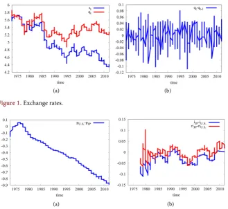
[image:4.595.210.540.313.615.2]

This paper studies the yen/dollar exchange rate for three reasons. First, Japan and the US are both large trading countries and their economy has a substantial weight in the world. Second, the yen/dollar exchange rate is among the few main currencies that have historical data, which serves the purpose well. Third, the studies on yen/dollar exchange rate abound, making it easy to compare. The short-run data spans from January 1973 to November 2012, taken on the first day of each month from “DataStream”.3

Figure 1 presents the nominal, real exchange rates and changes in the real exchange rates in the short-run. Figure 2 plots the price and interest rate diffe-rentials. September 1985 is tested to be a structural break following the proce-dures in [14], which is widely believed to be the consequence of the Plaza

(a) (b) Figure 1. Exchange rates.

(a) (b) Figure 2. Price and interest rate difference in logs.

3_{The specific time-series data consist of the following. S: yen/dollar exchange rate (New York market}

buying rates for the short run; close rates on the last day of each year for the long run); Ijp: Japanese

nominal interest rate level (euro rates in London market for the short run; 7-year government bond rate for the long run); Ius: U.S. nominal interest rate level (euro rates in London market for the short

run; 10-year government bond rate for the long run); Pus: U.S. consumer price index (CPI); Pjp:

Jap-anese CPI; infus: U.S. inflation level (calculated from “PU”); infjp: Japanese inflation level (calculated

from “PJ”); rius: U.S real interest level (calculated from “IU” and “INFU”); rijp: Japanese real interest

(5)

[image:5.595.225.538.275.331.2] [image:5.595.210.541.617.698.2]

DOI: 10.4236/me.2019.109129 2055 Modern Economy Accord. In the ADF test, the t-value is −2.2870, smaller in absolute terms than the 5-percent critical value −2.57. Similarly, unit root tests for UIP are per-formed, and the results are summarized in the following.

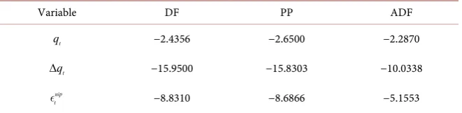
Table 1 indicates that absolute PPP fails, while relative PPP and UIP hold in the short-run.

2.2. Exchange Rate Determination

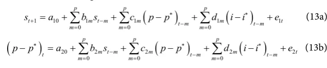
The success of relative PPP may lead someone to believe that the price differen-tial is enough to explain the movement of the nominal exchange rate. This sec-tion, however, argues that we should discard this optimistic idea. Assume that only the price differential between Japan and U.S. determines the Japanese no-minal exchange rate, then we can write out this as the following pth order

bi-variate vector autoregressive (VAR) system in its standard form:

(

)

(

)

10 1 1 1 1

1 1 1

p p p

t m t m m _{t m} m _{t m} t

m m m

s a b s c p p∗ d i i∗ e

− ₋ ₋

= = =

= +

∑

+

∑

− +

∑

− + (7a)

(

)

20 2 2

(

)

2

(

)

2

1 1 1

p p p

m t m m m t

t _m _m t m _m t m

p p∗ a b s c p p∗ d i i∗ e

− ₋ ₋

= = =

− = +

∑

+

∑

− +

∑

− + (7b)

where e1t and e2t are white-noise disturbances.

Equations (7a) and (7b) are called the restricted system in that all the coeffi-cients of interest differential, d1m and d2m are assumed to be zeros. The block

exogeneity test, however, reveals that this restriction is binding. The _χ2

dis-tributed test statistics is 50.6849, far exceeding the 1 percent critical value.4

Therefore the interest differential is essential in the determination of the ex-change rate in the short-run.

The above preliminary tests suggest that CHEER may be more appropriate to forecast the exchange rate in the short-run. Recall that the relative PPP and UIP are:

t t t t

s p p∗ q

∆ = ∆ − ∆ + ∆ _(8a)

1 uip

t t t t t

s s i i∗

+ − = − + (8b)

Differencing Equation (8b) yields

(

)

1 uip

t t t t t

s s i i∗

+

∆ − ∆ = ∆ − + ∆ (9)

and substituting Equation (8a) into Equation (9),

Table 1. Summary of the unit root tests.

Variable DF PP ADF

t

q −2.4356 −2.6500 −2.2870

t

q

∆ −15.9500 −15.8303 −10.0338

uip t

 −8.8310 −8.6866 −5.1553

4_{For lag length p, both SBC and AIC criteria selects 2. The number of restrictions thus in (7a) and}

(6)

DOI: 10.4236/me.2019.109129 2056 Modern Economy

(

) (

)

1

t t t t t t

s p p∗ i i∗

η

+

∆ = ∆ − + ∆ − + (10)

where uip

t qt t

η = ∆ + ∆ .

Equation (10) is the model of nominal exchange rate determination in the short-run. It states that the exchange rate is jointly determined by the price and interest rate differentials: the increases in either price or the interest rate diffe-rentials will cause the future nominal exchange rate to depreciate. For example, if a country is suffering higher inflation or sharp interest rate increasing, its ex-change rate will depreciate.

It is worth noting that, compared with normal CHEER approach, which usually searches cointegration directly between st, p pt− t∗ and i it− t∗,

Equa-tion (10) has two modificaEqua-tions. One is that it is of first-order difference, and the other is that it involves expectations, thought the expectations here are assumed to be perfect. Here we will show that the two modifications are necessary be-cause we cannot find cointegration with either modification absent. To see this, consider the following three models:

Model 1: st, p pt− t∗, i it− t∗

Model 2: st+1, p pt− t∗, i it− t∗

Model 3: ∆st+1, ∆

(

p pt− t∗

)

, ∆ −

(

i it t∗

)

.

Model 1 is the most often seen practice in most papers, which investigate the relationship between the exchange rate, price and interest rate differentials. Model 2 adds expectation, which comes from the UIP hypothesis. Model 3 is further modified by adding a first-order difference, which is based on the em-pirical tests of PPP and UIP. The results of the cointegration tests are summa-rized in Table 2. Comparing the results in Table 2, we conclude that the effect of the two modifications is significant. Only model 3, i.e., the model with expecta-tion and first-order difference can yield the cointegraexpecta-tion relaexpecta-tionship.5

2.3. The VAR Analysis

Model 3 implies that the short-run model can be presented by a structural VAR system

(

)

(

)

1 10 1 1 1 1 1

0 0 0

p p p

t m t m m _{t m} m _{t m} t

m m m

s a b s c p p∗ d i i∗ e

+ + − ₋ ₋

= = =

∆ = +

∑

∆ +

∑

∆ − +

∑

∆ − + (11a)

Table 2. Cointegration tests.

t

s , p pt t

∗

− _,i i_t₋_t∗

1

t

s+, p pt t

∗

− _,i i_t₋_t∗

1

t

s+

∆ _,

(

p pt t

)

∗

∆ − _,

(

i it t

)

∗

∆ −

Eigenv Maxλ trace Eigenv Maxλ trace Eigenv Maxλ trace

0.0679 20.84 39.78 0.0617 18.85 40.37 0.1487 47.51 87.52

0.0483 14.66 18.95 0.0562 17.11 21.52 0.0817 25.14 40.01

0.0144 4.29 4.29 0.0148 4.40 4.40 0.0492 14.88 14.88

5_{At the 5% level,} _Max_λ_{and Trace for}

0 0,1,2

H = _{are 21.07, 14.90, 8.18 and 31.52, 17.95, 8.18}

(7)

(

)

(

)

( )

20 2 1 2

0 0

2 2

0

p p

m t m m

t _m _m t m

p

m _{t m} t

m

p p a b s c p p

d i i e

∗ ∗ + − ₋ = = ∗ − = ∆ − = + ∆ + ∆ − + ∆ − +

∑

(11b)

(

)

30 3 1 3

(

)

3

(

)

3

0 0 0

p p p

m t m m m t

t _m _m t m _m t m

i i∗ a b s c p p∗ d i i∗ e

+ − ₋ ₋

(

p pt t∗

)

∆ − .

Moreover, considering the interest rate differential is small in value and diffe-rencing it may cause it to appear white noise, its effect tends to be underesti-mated in (10).6_{Granger causality test between}

1

t

s+ ,

(

p pt− t∗

)

and

(

i it− t∗

)

yields a different result, as is shown in Table 4.

As indicated from Table 4, in the 5 percent significance level, the price diffe-rential

per-cent of st+1 at the 12-lag ahead forecast, leaving

(

p pt− t∗

)

only account for

Table 3. Summary of the Granger causality tests in the short-run.

variable ∆st+1

(

p pt t

)

∗

∆ −

(

i it t

)

∗

∆ −

1

t

s+

∆ 22.5773 0.0000 0.4155 0.6603 1.2441 0.2893

(

p pt t

)

∗

∆ − 5.8880 0.0030 6.8310 0.0012 3.8305 0.0225

(

i it t

)

∗

∆ − 2.0701 0.1275 0.5540 0.5750 3.2553 0.0395

6_{The mean of}

(

)

t t

i i∗

(8)

[image:8.595.209.539.90.173.2]

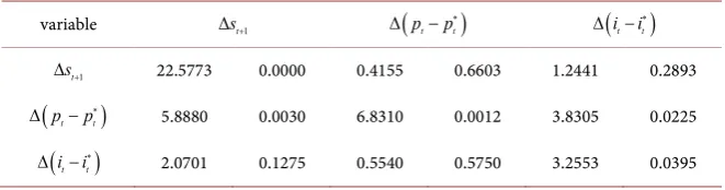
Table 4. Summary of the Granger causality tests.

variable st+1

(

p pt t

)

∗

−

(

i i_t₋_t∗

)

1

t

s+ 1277.61 0.000 0.6698 0.7804 2.2332 0.0101

(

p pt t

)

∗

− 1.2960 0.2185 21390.95 0.0000 2.4276 0.0048

(

i it t

)

∗

− 1.8415 0.0400 2.8121 0.0010 320.3485 0.0000

0.54 percent in the same period. Therefore, the interest differential seems more essential in the determination of exchange rate movement in the short run.

3. Long-Run Analysis

The long-run data from the year 1870 to 2012, consisting of the exchange rate, the CPI index and the long-term interest rates for the US and Japan.7_{Figure 3}

depicts the exchange rates and Figure 4 shows the price and interest rate diffe-rentials. [14] tests reveal that from 1870 to 2012, two structural breaks occurred. One is the year 1945, in which the yen depreciated more than 200 percent (from 4.29 to 15). The other notable break is the year 1970, in which the yen began to appreciate sharply due to the oil shock. We next proceed to test PPP and UIP, the same as the analysis for the short run. ADFs test of qˆ_t and uip

t

 yield the statistics of −2.93 and −3.30, respectively. Both statistics exceed the 5-percent critical value of −2.88. Therefore, both PPP and UIP hold in the long-run. Subs-titute st in Equation (1) into (5), and assuming perfect foresight, the long-run

exchange rate model can be written as:

(

) (

)

1

t t t t t t

s p p∗ i i∗

ξ

+ = − + − + (12)

where ξt is the sum of errors from PPP and UIP. The Johansen test results of

Equation (12) are summarized in Table 5.

)

(

)

1 10 1 1 1 1

0 0 0

p p p

t m t m m _{t m} m _{t m} t

m m m

s a b s c p p∗ d i i∗ e

+ − ₋ ₋

= = =

= +

∑

+

∑

− +

∑

− + (13a)

(

)

20 2 2

(

)

2

(

)

2

0 0 0

p p p

m t m m m t

t _m _m t m _m t m

p p∗ a b s c p p∗ d i i∗ e

− ₋ ₋

= = =

− = +

∑

+

∑

− +

∑

− + (13b)

7_{Long-term interest rates are U.S 10 year government bond yield and Japanese 7 year government}

[image:8.595.218.538.633.700.2]

(9)

[image:9.595.208.539.60.372.2]

(a) (b) Figure 3. Exchange rates.

(a) (b) Figure 4. Price and interest rate difference in logs.

Table 5. Summary of the Johansen cointegration test in the long-run.

Eigenv Maxλ Trace H r0: p r− Maxλ95 Trace95

0.1286 18.19 34.31 0 3 21.07 31.52

0.051 10.86 16.12 1 2 14.90 17.95

0.0192 5.26 5.26 2 1 8.18 8.18

(

)

30 3 3

(

)

3

(

)

3

0 0 0

p p p

m t m m m t

t _m _m t m _m t m

i i∗ a b s c p p∗ d i i∗ e

− ₋ ₋

= = =

− = +

∑

+

∑

− +

∑

∆ − + (13c)

where a, b, c and d are parameters, and eit (i=1,2,3) are error-terms.

Granger causality tests are performed to answer the first question. The joint F-statistics and the significance levels of system (13a) through (13c) are reported in Table 6.8 _{Table 6}_{indicates that at 5 percent significance level,}

1

t

is not an endogenous

va-riable in the system of exchange rate determination.

To answer the second question, the block exogeneity test, which is similar to the method in (7a) and (7b) is conducted.9_{The likelihood ratio statistics is}

8_{Both AIC and SBC select the lag length 3.}

9_{Here the number of restrictions is 10 (lag 0, 1, 2, 3, 4 in each equation) and the unrestricted model}

(10)

[image:10.595.209.539.90.168.2]

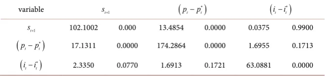
Table 6. Summary of the Granger causality tests in the long-run.

variable st+1

(

p pt− t∗

)

(

i it−t∗

)

1

i it − t∗

)

, is trivial and CHEER hypothesis fails in the

long run. The failure of CHEER in the long run seems puzzling here because we have found cointegration in the short run and many economic hypotheses tends to hold better in the long run. [15], for example, is unable to find cointegration in the short run but finds cointegration in the long run.10_{We can explain the}

puzzle from the history of financial markets. Financial markets did not develop well until the past 30 years and its role in the exchange rate determination is not apparent if we view it in a very long data span. If we test CHEER hypothesis us-ing the recent data, the interest rate differential tends to become more significant because of its notable size. In short, the 140 years is too long and the effect of fi-nancial market in exchange rate determination in recent years is “diluted”.11

4. Conclusion

This paper tests CHEER approach both in the short-run and the long-run with the yen/dollar exchange rate. The main result is that CHEER approach is only supported by the short-span data. Actually, it is revealed that the interest rate differential plays a more important role in the exchange rate determination. When examined in the historical data, the price level difference alone becomes sufficient to explain the exchange rate movement and CHEER fails. The reason behind this is the different stage of the international financial market. Since the core idea of CHEER is to determine the exchange rate from both goods market and financial market, it is not a surprise that it will fail during the period when at most times, the international financial market is under-developed, compared to the goods market.

Acknowledgements

This paper is sponsored by the National Natural Science Foundation of China. I

10_[15]_{researched on yen/dollar case and found no causality between prices and exchange rates in the}

short run. However, causality is found running from relative prices to exchange rates along with in-terest rates in the long run.

11_{The forecast error decomposition also suggests that the price differential}

(

)

t t

p p₋ ∗

is the domi-nant factor in the determination of st+1. In the 5-lag ahead forecast horizon,

(

p pt t

)

∗

− explains

8.495 percent of the error of st+1, while

(

i it t

)

∗

(11)

DOI: 10.4236/me.2019.109129 2061 Modern Economy would like to thank Nikolay Gospodinov, Artem Prokhorov and Hiroshi Shibuya for insightful comments and suggestions. All errors remain my own. 130 Mei-long Road, Shanghai, China.

Conflicts of Interest

The authors declare no conflicts of interest regarding the publication of this pa-per.

References

[1] Cassel, G. (1920) Further Observations on the World’s Monetary Problem. The Economic Journal, 30, 39-45.https://doi.org/10.2307/2223193

[2] MacDonald, R. (2000) Concepts to Calculate Equilibrium Exchange Rates: An Overview. Discussion Paper Series 1: Economic Studies 2000, 03, Deutsche Bun-desbank, Research Centre, Frankfurt.

[3] Juselius, K. (1991) Long-Run Relations in a Well-Defined Statistical Model for the Data Generating Process. Cointegration Analysis of the PPP and the UIP Relations for Denmark and Germany. In: Econometric Decision Models: New Methods of Modeling and Applications: Proceedings of the 2nd International Conference on Econometric Decision Models, Vol. 366, Springer, Berlin, 336.

https://doi.org/10.1007/978-3-642-51675-7_20

[4] Johansen, S. and Juselius, K. (1992) Testing Structural Hypotheses in a Multivariate Cointegration Analysis of the PPP and the UIP for UK. Journal of Econometrics, 53, 211-244.https://doi.org/10.1016/0304-4076(92)90086-7

[5] Caporale, G.M., Kalyvitis, S. and Pittis, N. (2001) Testing for PPP and UIP in an FIML Framework: Some Evidence for Germany and Japan. Journal of Policy Mod-eling, 23, 637-650.https://doi.org/10.1016/S0161-8938(01)00078-3

[6] Keblowski, P. and Welfe, A. (2010) Estimation of the Equilibrium Exchange Rate: The Cheer Approach. Journal of International Money and Finance, 29, 1385-1397. https://doi.org/10.1016/j.jimonfin.2010.03.007

[7] Giannellis, N. and Koukouritakis, M. (2013) Exchange Rate Misalignment and In-flation Rate Persistence: Evidence from Latin American Countries. International Review of Economics & Finance, 25, 202-218.

https://doi.org/10.1016/j.iref.2012.07.013

[8] Meese, R. and Rogoff, K. (1988) Was It Real? The Exchange Rate-Interest Differen-tial Relation over the Modern Floating-Rate Period. The Journal of Finance, 43, 933-948.https://doi.org/10.1111/j.1540-6261.1988.tb02613.x

[9] Campbell, J.Y. and Clarida, R.H. (1987) The Dollar and Real Interest Rates. Carne-gie-Rochester Conference Series on Public Policy, 27, 103-139.

https://doi.org/10.1016/0167-2231(87)90005-4

[10] Edison, H.J. and Pauls, B.D. (1993) A Re-Assessment of the Relationship between Real Exchange Rates and Real Interest Rates: 1974-1990. Journal of Monetary Eco-nomics, 31, 165-187.https://doi.org/10.1016/0304-3932(93)90043-F

[11] Juselius, K. and MacDonald, R. (2004) International Parity Relationships between the USA and Japan. Japan and the World Economy, 16, 17-34.

https://doi.org/10.1016/S0922-1425(03)00003-3

(12)

[13] Gokcan, A. and Ozmen, E. (2002) Erc Working Papers in Economics 01/01. [14] Lee, J. and Strazicich, M.C. (2003) Minimum Lagrange Multiplier Unit Root Test

with Two Structural Breaks. Review of Economics and Statistics, 85, 1082-1089. https://doi.org/10.1162/003465303772815961

[15] Cheng, B.S. (1999) Beyond the Purchasing Power Parity: Testing for Cointegration and Causality between Exchange Rates, Prices, and Interest Rates. Journal of Inter-national Money and Finance, 18, 911-924.