Testing the stability of supersonic ionized Bondi accretion flows with radiation hydrodynamics

arXiv:1903.00479v1 [astro-ph.SR] 1 Mar 2019

Testing the stability of supersonic ionized Bondi accretion

flows with radiation hydrodynamics

Bert Vandenbroucke,

Nina S. Sartorio,

Kenneth Wood,

Kristin Lund,

Diego Falceta-Gon¸calves,

Thomas J. Haworth,

Ian Bonnell,

Eric Keto,

Daniel Tootill,

1_{SUPA, School of Physics & Astronomy, University of St Andrews, North Haugh, St Andrews, KY16 9SS, United Kingdom}

2_{Instituto Nacional de Pesquisas Espaciais - INPE, Divis˜ao de Astrof´ısica, Av. dos Astronautas, 1.758 - S˜ao Jos´e dos Campos - SP, Brazil} 3_{Escola de Artes, Ciˆencias e Humanidades, Universidade de S˜ao Paulo, Rua Arlindo Bettio 1000, S˜ao Paulo, SP, 03828-000, Brazil} 4_{Astrophysics Group, Imperial College London, Blackett Laboratory, Prince Consort Road, London SW7 2AZ, UK}

5_{Harvard-Smithsonian Center for Astrophysics, Cambridge, MA 02138, USA}

Accepted XXX. Received YYY; in original form ZZZ

ABSTRACT

We investigate the general stability of 1D spherically symmetric ionized Bondi accre-tion onto a massive object in the specific context of accreaccre-tion onto a young stellar object. We first derive a new analytic expression for a steady state two temperature solution that predicts the existence of compact and hypercompact Hii_{regions. We then}

show that this solution is only marginally stable if ionization is treated self-consistently. This leads to a recurring collapse of the Hii_{region over time. We derive a semi-analytic}

model to explain this instability, and test it using spatially converged 1D radiation hydrodynamical simulations. We discuss the implications of the 1D instability on 3D radiation hydrodynamics simulations of supersonic accreting flows.

Key words: methods: numerical – hydrodynamics – radiation: dynamics – instabil-ities – HII regions

1 INTRODUCTION

The problem of a spherically symmetric accretion flow onto a massive star including a rigorous treatment of the hydro-dynamics was first introduced byBondi(1952), and is con-sequently referred to as the Bondi problem.Mestel (1954) studied the effect of ionizing radiation on the original Bondi problem, using an approximation whereby both the ion-ized and the neutral region are assumed to be isothermal, with different isothermal sound speeds and a sharp transi-tion from ionized to neutral regime at the ionizatransi-tion front.

Keto(2002,2003) showed that this work explains the exis-tence of a steady state solution in which an ionized region is trapped inside the accreting flow. This explains the ex-istence of trapped compact and ultracompact Hiiregions around massive accreting stars. These ultracompact Hii re-gions are indeed observed around massive protostars, with observed size estimates varying from∼103_{AU (Churchwell}

2002) to as small as ∼ 10 AU (Ilee et al. 2016). He also showed how accretion can continue while the protostar is

⋆ _{E-mail : [email protected]}

already emitting UV radiation, which has implications for the final mass of a young stellar object.

Recently, this work was extended to 3D using a Monte Carlo radiation hydrodynamics code (Lundet al., submit-ted to MNRAS). They were able to numerically simulate a trapped Hiiregion, and also showed the change in regime from a trapped R type ionization front into an expanding D type ionization front under a changing source luminos-ity, with the subsequent shut down of accretion onto the central star. However, their work also casted doubt about the stability of the steady state solution ofKeto(2002), as their trapped Hiiregions showed signs of periodic collapse, whereby the ionization front periodically collapsed onto the central star and moved outwards again.

In this work, we will analyse this instability in more detail, using a high resolution 1D spherically symmetric ra-diation hydrodynamics code, and a semi-analytic stability analysis.

Note that massive stars are expected to form through an accretion disk (Beltr´an & de Wit 2016;Kuiper & Hosokawa 2018), which leads to more extended ultracompact Hii re-gions, and stabilises the ionization front (Sartorioet al, sub-mitted to MNRAS). This renders the assumption of

cal symmetry an unlikely scenario for accretion onto a pro-tostar. Nevertheless, this work is still relevant for our un-derstanding of trapped Hii_{regions and can serve as a} use-ful benchmark test for models that combine hydrodynamics, photoionization and gravitational accretion.

2 ANALYTICS

In this section, we present the analytical solution to the orig-inal Bondi problem, and the extended Bondi problem with ionizing radiation. This work is a summary of the original work ofBondi(1952) on steady state accretion, and extends the work ofMestel(1954) andKeto(2002) with a full ana-lytic expression for two temperature steady state accretion. We will summarize the main equations and present the full analytic steady state solution, before addressing the stability of this analytic solution under self-consistent ionization.

2.1 Bondi accretion

We assume spherically symmetric flow onto a massive object of constant mass M with a constant accretion rate (Bondi 1952)

˙

Ma= 4πr2ρ(r)v(r), (1)

withρ(r) andv(r) the mass density and fluid velocity as a function of radiusr.

If we furthermore neglect the gravitational force due to the mass of the accreting fluid and assume the potential is dominated byM, and assume an isothermal equation of state with a constant sound speedcs(r) =p

dP(r)/dρ(r) = Cs, the constancy of the accretion rate leads to a specific form of Bernoulli’s equation:

v2_(r) 2C2

s

+ ln (ρ)−2RB_r = constant, (2)

where we introduced the (constant) Bondi radius

rB(r) = GM 2c2

s(r)

=RB (3)

≈110.9

_M

M⊙

Cs 2 km s−1

−2

AU, (4)

withG= 6.674×10−11m3 kg−1 s−2 Newton’s constant. Assuming that the velocity vanishes at infinity, we find the value of the constant:

v2(r) 2C2

s

+ ln (ρ)−2RB_r = ln (ρ∞), (5)

withρ∞the rest density of the accreting material. By eval-uating this equation atr=RB, we can find the densityρB at the Bondi radius:ρB=e3/2_{ρ∞≈4.48ρ∞.}

Using (1), we find an expression for the density as a function of radius:

ρ(r) =−ρBR

2 BCs

r2_v(r) . (6)

Substituting this in (5), we find

v(r)

Cs 2

−ln "

v(r)

Cs

2#

−4 ln

r RB

+ 3−4RB

r = 0, (7)

which has general solution (Cranmer 2004)

v(r) =−Cs v u u

t−W −

RB

r 4

exp

3−4RB r

!

, (8)

whereW(x) is the Lambert W function, and the negative root was chosen since we want material to be accreting onto the central object.

The Lambert W function is a complex valued func-tion with an infinite number of branches, but two of these branches,W0(x) andW−1(x), are real valued in the range [−1/e,0], withW0(−1/e) =W−1(−1/e) =−1,W0(0) = 0, andW−1(x)→ − ∞forx→0. Since we want the velocity to be a strictly increasing function of radius, we see that we start on theW0 branch forr > RB, and switch to theW−1 branch atr=RB. Forr→0, the velocity diverges.

We end up with the following analytic expressions for the velocity for steady state accretion onto a massive object:

v(r) = (

−Csp−W−1(−ω(r)) r≤RB,

−Csp

−W0(−ω(r)) r > RB, (9) with

ω(r) =

RB r

4 exp

3−4RB r

. (10)

2.2 Ionizing radiation

To include ionization from a central isotropic point source, we followMestel(1954) and assume a sharp transtion from ionized to neutral at a well defined radiusRI. Both inside and outside the ionized region the gas obeys an isothermal equation of state, with the constant sound speed given by Cs,iandCs,n respectively. We will characterize the change in equation of state in terms of thepressure contrast Pc = C2

s,i/Cs,n2 . Since the temperature in the ionised region will be higher than that in the neutral region, we always have Cs,i> Cs,n, and hencePc>1.

Since (6) and (9) are completely determined by the boundary condition atr→+∞, this solution is still valid for r≥RI, with Cs =Cs,n, andRB =RB,n =GM /(2C2

s,n). To find the solution forr < RI, we impose conservation of mass and momentum across the ionization front to find the following Rankine-Hugoniot conditions:

ρi(RI)vi(RI) =ρn(RI)vn(RI) (11)

ρi(RI) vi2(RI) +Cs,i2

=ρn(RI) vn2(RI) +Cs,n2

, (12)

whereρi(r) andvi(r), andρn(r) andvn(r) are the density and velocity in the ionized and neutral regions respectively.

If we introduce thejump factor

Γ = ρi(RI) ρn(RI) =

vn(RI)

vi(RI), (13)

we find the following equation for the jump as a function of the known neutral velocityvn(RI):

Cs,i2 Γ2− v2n(RI) +Cs,n2

Γ +v2n(RI) = 0, (14)

with solutions

Γ = 1 2C2

s,i

v2n(RI) +Cs,n2

±

q v2

n(RI) +Cs,n2 2

−4C2 s,ivn2(RI)

Γ only has real solutions for|vn(RI)| ≥vRor|vn(RI)| ≤

vD(note thatvn(r) is always negative because we are in an accretion regime), with

vR=Cs,i 

1 + s

1−

_Cs,n

Cs,i

2

, (16)

vD=Cs,i 

1− s

1−

Cs,n

Cs,i

2

, (17)

which are commonly referred to as the R type and D type solutions. We will limit ourselves to R type solutions. In the region between the R type and D type solutions there is no solution with a single shock at the position of the ioniza-tion front, but more complex double front soluioniza-tions could be possible; we do not study these in this work.

It is obvious that|vn(RI)|> Cs,i, so that the R type solution implies supersonic neutral gas at the ionization front. Furthermore, Γ>1 for|vn(RI)| ≥vR, which implies

|vi(RI)|<|vn(RI)|.

Γ has two solutions in the R type region, corresponding to a large and a small jump (corresponding to the positive and negative sign in (15)). We call these theweakandstrong R type solution. If we assume a density structure that ini-tially evolved through Bondi accretion without ionization, then the solution will naturally evolve into the weak solu-tion with the smallest jump, and this is the solusolu-tion we will assume below. In this case, the velocity in the ionized re-gion will also be supersonic (see AppendixAfor a detailed analysis of weak and strong R type solutions and imposed velocity restrictions).

Inside the ionized region, equation (1) still gives us the density:

ρi(r) = ρi(RI)R 2 Ivi(RI)

r2_vi(r) . (18)

The Bernoulli equation (2) now becomes

v2 i(r) 2C2

s,i

+ ln (ρi(r))−_CGM2 s,ir

=

v2 i(RI) 2C2

s,i

+ ln (ρi(RI))−_RIGM_C2 s,i

, (19)

since we now need to apply boundary conditions atr=RI instead ofr→ +∞.

Similarly as before, we can combine this equation with (6) to get

vi(r)

Cs 2

−ln "

vi(r)

Cs

2#

−4 ln

r RI

+ ln

v2

i(RI) C2

s,i

−4RB,i

r −

v2 i(RI)

C2 s,i

+ 4RB,i

RI = 0, (20)

where we introduced the Bondi radius for the ionized region RB,i=GM /(2Cs,i2 ). This equation has the general solution

vi(r) =−Cs,ip−W(−ωi(r)), (21)

10−17

10−16

ρ

(g

cm

−

3)

30 AU 40 AU 50 AU

ρ∼r−1.4

20 40 60 80 100

r(AU)

−50 −40 −30 −20

v

(k

m

s

−

1)

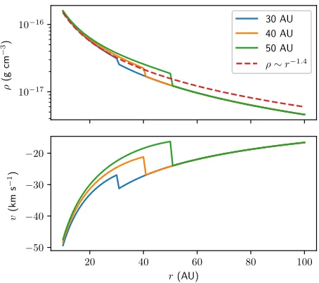
Figure 1.Density (top) and velocity (bottom) as a function of radius for the analytic two temperature solution for three different values of the ionization radiusRI, as indicated in the legend. All models used a central mass M = 18 M⊙, a pressure contrast Pc = 32, a Bondi density ρB = 10−19 g cm−3 and a neutral sound speedCs,n= 2.031km s−1. The dashed line on the top panel shows a power law approximation for the density profile in the ionized region.

with

ωi(r) =

RI r

4

vi(RI) Cs,i

2

exp

4RB,i RI −4

RB,i

r −

v2 i(RI)

C2 s,i

. (22)

Note that as in the neutral case, this solution will switch from theW0 to theW−1 branch at a critical radiusRc, for whichvi(Rc) =−Cs,i. However, we know that this cannot happen for a weak R front, asvi(r)<−Cs,i. We hence only need to consider theW−1 branch.

The full solution for spherically symmetric accretion with ionization (in the case|vn(RI)| ≥vR) is:

ρ(r) = (

ρn(r) r > RI,

ρi(r) r < RI, (23)

v(r) = (

vn(r) r > RI,

vi(r) r < RI, (24)

with

ρn(r) =−ρB,nR

2 B,nCs,n

r2_vn(r) , (25)

ρi(r) =ρi(RI)R 2 Ivi(RI)

r2_vi(r) , (26)

and

vn(r) = (

−Cs,np

−W−1(ωn(r)) r≤RB,n,

−Cs,np

with

ωn(r) =−

RB,n

r 4

exp

3−4RB,n r

, (29)

ωi(r) =−

RI

r

4

vi(RI) Cs,i

2

(30)

exp

4RB,i RI −4

RB,i

r −

v2 i(RI)

C2 s,i

. (31)

The parameters ρi(RI) and vi(RI) are given by the jump conditions:

ρi(RI) = Γρn(RI), (32)

vi(RI) = vn(RI)

Γ , (33)

with

Γ = 1 2

v2 n(RI)

C2 s,i

+ 1 Pc −

s

v2 n(RI)

C2 s,i

+ 1 Pc

2

−4v2n(RI) C2

s,i !

,

(34)

so that the entire solution is parametrised in terms of Pc, RI,ρB,n,Cs,nandM.

The density and velocity profile of the two temperature solution is plotted in Fig.1for three different values of the ionization radius RI. It can be seen that higher values of RI lead to higher densities and lower velocities inside the ionised region; the solution in the neutral region is the same for all models.

2.3 Self-consistent ionization

The derivation above did not make any assumptions about how the ionization happens, and just assumed ionization leads to a constant ionization radiusRI. However, in general, the ionization radiusRI(t) will vary with time, and the time evolution will be linked to the hydrodynamical quantities, ρ(r, t) and v(r, t). To find out if the steady-state solution obtained above is actually stable, we have to include this effect.

For simplicity, we will assume that the dynamical time scale tdynover which the hydrodynamical quantities evolve is much larger than the recombination time scale, trec = (nHαB(T))−1_{, wherenHis the number density of hydrogen} atoms and αB(T) is the collisional recombination rate of ionized hydrogen to all excited levels of neutral hydrogen, but excluding ionizations to the ground state (the so-called on-the-spot approximation), which depends on the temper-atureT. Under this assumption, the ionization structure of the system instanteneously adapts to any change in density, and we can model ionization by simply changing the equa-tion of state.

To get the ionization radius RI, we use a Str¨omgren approximation, and assume that all material inside the ion-ization region is completely ionized. At the ionion-ization radius, we have a strong discontinuity, and outside the ionization ra-dius the material is completely neutral. In this case, the ion-ization balance equation is given by (Osterbrock & Ferland 2006)

Q(t) = 4π Z RI(t)

Rc

n2H(r, t)αB(T)r2dr, (35)

whereQ(t) is the total ionizing luminosity of the star. Since the steady state density profile is very centrally peaked, and since we do not realistically expect the profile to keep up untilr = 0, we also introduced an inner cut off radiusRc, below which we assume no more ionizations to occur.

Under the two temperature approximation, the recom-bination rateαB(Ti) =αiis constant. If we further assume our gas to be composed of hydrogen only, we can rewrite the ionization balance equation as

Q(t) = 4παi m2

H ZRI(t)

Rc

ρ2(r, t)r2dr, (36)

wheremH= 1.674×10−27 kg is the hydrogen atomic mass. Taking the time derivative of this equation, we find the fol-lowing equation for the time evolution ofRI(t):

dRI(t) dt =

1 ρ2_{(RI(t), t)R}2

I(t) "

m2 H 4παi

dQ(t) dt −2

Z RI(t)

Rc

ρ(r, t)∂ρ(r, t) ∂t r

2 dr

# , (37)

where we assumed the ionization radius is a continuous func-tion of time, and used the general form of Leibniz’ rule:

d dx

Z b(x)

A

f(x, y)dt !

=

f(x, b(x))d dxb(x) +

Z b(x)

A ∂

∂xf(x, t)dt. (38)

2.4 Stability analysis

For what follows, we will assume a constant source luminos-ityQ(t), and assume we already have a steady state solution as derived in2.2. We will now perturb this solution by intro-ducing a small density perturbation outside the ionization radius. As shown by (37), this will not affect the ionization radius, and the perturbation will accrete until it reaches the ionization front radius. Once it reaches the ionization front and crosses it by a small distance ε, the ionization front radius will change according to

dRI(t) dt =−

2 ρ2_{(RI(t), t)R}2

I(t) Z RI(t)

RI(t)−ε

ρ(r, t)∂ρ(r, t) ∂t r

2_{dr, (39)}

since this is the only part of the integral that is non trivial. This expression does not lend itself to a rigorous linear per-turbation analysis because of the presence of an integral in a differential equation, so that we will restrict ourselves to a semi-analytic analysis below.

What happens next depends on the sign of∂ρ(r, t)/∂t. If this sign is positive (a positive perturbation), the value of the integral will be positive and the ionization front will move inwards. For a negative perturbation, the ionization front will move outwards.

dynamic equilibrium value, or will keep moving in the same direction. In the limit of a very large positive perturbation, the ionization front will move with the accreting bump and collapse entirely. This qualitative behaviour of the ionization front radius constitutes a first important result:the change in ionization front caused by a perturbation cannot be un-done while that perturbation is still present inside the

ion-ized region. The rate at which the ionization radius changes

depends on the size and the shape of the perturbation. Once the initial perturbation leaves the ionized region by crossing the cut off radiusRc, the situation is nominally reset to the original two temperature situation. However, since the profile behind the perturbation adjusted to a new ionization radius while the perturbation was still present, the amount of available material to ionize will now no longer match the initial, stable two temperature solution. For a pos-itive perturbation, the ionization front will have shrunk and the density will now be too low; for a negative perturba-tion the reverse will have happened. We now end up in the opposite scenario of what we started out with: the initially positive perturbation now results in a profile with a nega-tive perturbation, while the initially neganega-tive perturbation is now a positive perturbation. This is a second important result:once a perturbation leaves the ionized region, a new

perturbation of opposite sign is created.

The new perturbation of opposite sign has to ensure the ionizing luminosityQ(t) is exactly balanced by recombina-tions (see (36)). Since the new perturbation will be created at a larger radius than the original perturbation, and since the Bondi accretion profile for the density scales as∼r−1.4, a larger density perturbation is needed to achieve this. This leads to the final important result:the newly created

pertur-bation will always be larger than the original perturpertur-bation.

In conclusion, any initially small perturbation will lead to an oscillation of the ionization front radius on a time scale of the free fall time (the time a perturbation created at the ionization front needs to reach the inner cut off ra-dius) and with a growing amplitude, until the amplitude is large enough to cause the ionization front to move at the same speed as the perturbation. Physically, there are four interesting scenarios, depending on the sign and the size of the initial perturbation:

(i) A large positive perturbation will cause a collapse of the ionization front whereby the ionization front gets trapped inside the perturbation and collapses onto the cen-tral cut off radius.

(ii) A small positive perturbation will initially cause a collapse of the ionization front, but the ionization front will move at a slower pace than the accretion velocity of the per-turbation. When the perturbation reaches the central cut off radius, the ionization front will go through a phase of expan-sion, followed by one or more subsequent oscillations with growing ionization front speed, until the ionization front gets trapped inside a perturbation.

(iii) A large negative perturbation will initially cause an expansion of the ionization front until the perturbation reaches the central cut off radius. At this point the ion-ization front will collapse as in the case of a large positive perturbation.

(iv) A small negative perturbation will initially cause an expansion of the ionization front, followed by multiple

oscil-lations with growing ionization front speed, until the ioniza-tio front gets trapped inside a perturbaioniza-tion.

In the next section, we will test our semi-analytic stabil-ity analysis by numerically seeding known perturbations of a given sign and size that correspond to these four scenarios.

3 NUMERICAL SIMULATIONS

3.1 1D code

3.1.1 Algorithm

We use a textbook (Toro 2009) implementation of a 1D spherically symmetric second order finite volume method1_. We use a very conservative version of the slope limiter of

Hopkins(2015). Fluxes are estimated using an HLLC Rie-mann solver (Toro 2009) with a polytropic indexγ= 1.001 (we tested our results against an exact Riemann solver), and are limited using the per-face slope limiter ofHopkins

(2015). After every time step the pressure is reset using the isothermal equation of state, effectively mimicking the use of an isothermal Riemann solver. The spherical source terms needed to make the method spherically symmetric are added using a second order Runge-Kutta method, as suggested by

Toro(2009).

Gravity is added as an extra source term in the mo-mentum equation, using an operator splitting method that uses a leapfrog scheme (Springel 2010). We assume that the central mass is much larger than the total mass of the fluid, such that we only consider the mass of the central object, as an external force.

We know from Section2that the central density is di-vergent, which will cause our numerical method to break down for small radii. We therefore set up an inner boundary radius with outflow boundary conditions, inside which we do not follow the hydrodynamics. At a much larger radius, we set up an inflow boundary where we impose the constant accretion rate.

To include ionization, we assume the Str¨omgren approx-imation introduced above, so that the ionization radius is determined by finding the root of the following function:

fion(RI) =

X

j,rj<RI ρ2j

1 3

rj+1

2∆r

−

rj−1₂∆r 3

−Q′, (40)

whererj is the central radius of cellj;ρj is its density. ∆r is the radial size of a single cell, while

Q′ = m

2 HQ

4παB(Ti)−Qinner (41)

is the ionizing luminosity that makes it out of the inner mask (we will treatQ′ _{as a simulation parameter).}

Once the ionization radius is found, we set the pres-sure of the region based on the following adapted isothermal equation of state:

P(r) =ρ(r) (

C2

s r >=RI, C2

sPc r < RI,

(42)

10−21 10−18 10−15

ρB,n(g cm−3)

1043

1048

1053

Qi

(s

−

1)

10−4 10−1 102

trec(yr)

Figure 2. Ionizing luminosity as a function of neutral Bondi density (top), and as a function of ionization front recombination time (bottom) for a fixed central mass, pressure contrast, neutral sound speed and ionization front radius, assuming an inner cut off radiusRc= 10 AU and an ionization front radiusRI= 30 AU. The dashed lines correspond to the specific choice ofρB,nwe will use for our simulations.

where Pc is the pressure contrast between the ionized and neutral region that was introduced in Section2.

3.1.2 Simulation parameters

We want to set up physically plausible initial conditions for which our assumptions hold, i.e. we want the density to be high enough to guarantee trec << tdyn, while at the same time having a density that is low enough to actually be ion-ized by a physically plausible input luminosity Q′

. For a central stellar mass of 18 M⊙, we expect an ionizing lumi-nosityQi∼1048s−1(Keto 2003;Sternberg et al. 2003). For the steady state solution, the ionization balance equation is given by

Qi=4παiρ 2

i(RI)R4Ivi2(RI) m2

H

Z RI

Rc 1 r2_v2

i(r)

dr. (43)

We have to numerically integrate this equation to find the ionizing luminosity that corresponds to a given set of two temperature Bondi parameters.

Fig. 2 shows the ionizing luminosity Qi as a func-tion of the neutral Bondi density ρB,n, for a central mass M = 18 M⊙, neutral sound speed Cs,n = 2.031 km s−1 (corresponding to a hydrogen only gas with Tn = 500 K), pressure contrastPc= 32 (corresponding to an ionized tem-perature Ti = 8000 K), and assuming an ionization front radius RI = 30 AU (similar to Lund et al., submitted to

MNRAS) and inner cut off radius Rc = 10 AU (due to

numerical precision issues, we cannot compute the argu-ment to the Lambert W function for radii <∼ 10 AU). Also shown is the corresponding recombination time scale at the ionization front, computed as Td=mH/(ρn(RI)αi), with αi = 4×10−13 cm3 s−1. For realistic ionizing lu-minosities ∼ 1048 _s−1_{, we find a neutral Bondi density}

∼ 10−19 _{g cm}−3_{, and a corresponding recombination time} scale∼10−2 _{yr. At the ionization radius, the free fall time} is Tf f = p

2R3

I/(GM) = 8.723 yr (the free fall time tak-ing into account the Bondi velocity as initial velocity is of the same order of magnitude), so the recombination time is more than a factor 100 smaller than the typical dynamical time in the entire ionized region.

We also tested this assumption using an expensive 1D

10−17

10−16

ρ

(g

cm

−

3)

t= 0 yr t= 5 yr t= 10 yr t= 40 yr

20 40 60 80 100

r(AU)

−50 −40 −30 −20

v

(k

m

s

−

1)

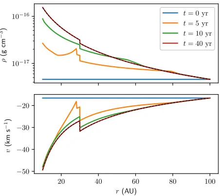
Figure 3.Density and velocity profile for the steady state solu-tion set up run at 4 different times throughout the simulasolu-tion, as indicated in the legend. The dashed line shows the analytic two temperature solution for the same parameters.

time dependent Monte Carlo radiation transfer algorithm (Tootill,private comm.) and found an excellent agreement between the time dependent results and the results obtained by assuming instanteneous ionization.

In what follows, we will hence use a neutral Bondi den-sityρB,n= 10−19_{g cm}−3_{. We will use a simulation box that} spans fromRc = 10 AU toRm= 100 AU, subdivided into 2700 equal sized radial cells, such that our desired ionization radius is on a cell boundary.

3.1.3 Stable solution

As a first test of the 1D code, we will try to obtain the sta-ble two temperature solution derived in Section2, starting from a constant density and velocity, and setting a constant ionization front radiusRI = 30 AU. The analytic solution is entirely fixed by specifying the neutral Bondi parameters, ionization front radius and pressure contrast; similarly the numerical solution should be entirely determined by the in-flow boundary conditions at Rm, the mass of the external point mass, and the ionization front position and pressure contrast if we do not restrict the solution atRc (which we can effectively do by using open boundaries). As initial con-ditions, we hence set ρ(r) = ρn(Rm) and v(r) = vn(Rm) everywhere.

10−7

10−6

10−5

10−4

10−3

|

ρs

−

ρa

|

/

|

ρs

+

ρa

|

20 40 60 80 100

r(AU)

10−7

10−5

10−3

|

vs

−

va

|

/

|

vs

+

va

|

Figure 4. Relative difference between the simulation and the analytic solution for the two temperature Bondi accretion with ionization and a constant ionization front radius, at the final sim-ulation timet= 40 yr.

10−17

10−16

ρ

(g

cm

−

3)

t= 10 yr t= 20 yr t= 40 yr t= 80 yr

20 40 60 80 100

r(AU)

−50 −40 −30 −20 −10

v

(k

m

s

−

1)

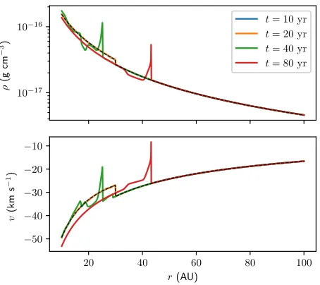
Figure 5.Density and velocity profile for the stability test run at 4 different times throughout the simulation, as indicated in the legend. The dashed line shows the analytic two temperature solution for the same parameters.

3.1.4 Stability test

As a second test, we test the stability of the steady state solution when the ionization front radius is computed self-consistently. To this end, we use the steady state output of the previous test, and compute the ionization radius based on equation (40).

Fig. 5 shows the resulting density and velocity pro-files at four different times during the simulation. Initially,

0 20 40 60 80

t(yr) 20

40

RI

(A

U

)

Figure 6.Ionization front radius as a function of time for the stability test run with self-consistent ionization. The dashed hor-izontal line shows the initial ionization front radius, while the full horizontal line shows the inner outflow boundary radius.

the steady state solution is stable. However, after∼10 yr, the density around the ionization front starts to break up into small peaks that travel inwards with the accretion flow. These small peaks cause tiny fluctuations in the ionization front radius, which gradually grow. After∼20 yr, the ioniza-tion front radius is no longer stable, and starts to oscillate, as can been seen from Fig.6.

It is important to note that we did not seed the small oscillations that lead to the collapse of the steady state so-lution; these oscillations are seeded numerically by accumu-lated round off error. We conclude that the steady state solution is only marginally stable, as even very small scale noise can cause it to become unstable.

3.1.5 Convergence

The result for the stability test discussed above depends on numerically seeded noise, which depends on resolution. This makes it impossible to perform a standard convergence test to check whether the time evolution of the ionization front corresponds to a physical effect or is simply caused by nu-merical issues. To show that our results do converge, we have to modify our set up so that we can obtain results that are independent of the spatial resolution for a sufficiently high spatial resolution. We identify two issues that need to be ad-dressed: (a) we need to seed the initial collapse of the ioniza-tion front with a known perturbaioniza-tion that is the same for all resolutions, (b) we need to make sure that newly created in-stabilities that cause the recurring collapse of the ionization front are consistent between resolutions. Since these depend on the shape of the ionization front, we need to make sure we resolve the ionization front consistently between resolutions. To obtain a spatially resolved ionization front, we con-vert the strong jump into a smooth linear transition. As be-fore, we compute the ionization front radiusRI from equa-tion (40). However, now the neutral fractionxH(r) of the gas does not just jump from 0 to 1 across the ionization front, but is given by

xH(r) =   

 

0 r < RI− 3 4S, xH,t(r) RI− 3

4S ≤r≤RI+ 3 4S, 1 r > RI+ 3

4S,

(44)

10−17

10−16

ρ

(g

cm

−

3)

W= 1AU W= 2AU

20 40 60 80 100

r(AU)

−50 −40 −30 −20 −10

v

(k

m

s

−

1)

W= 3AU

W= 4AU

W= 5AU

25 30 35

2×10−17

3×10−17

4×10−17

25 30 35

−32.5 −30.0 −27.5

Figure 7.Steady state density and velocity as a function of ra-dius for simulations with a smooth transition from ionized to neutral. The full lines show 2700 cell simulation results, with the width of the corresponding smooth transition indicated in the legend. The dashed line is the analytic two temperature solution. The insets show a zoom of the region around the ionization front radius, where the smooth simulations deviate from the analytic solution.

order polynomial:

xH,t(r) =−16₂₇S3(r−RI)3+S(r−RI) +1

2. (45) This particular transition shape was chosen because it al-lows us to control the slope of the transition, while en-suring continuous first derivatives in the transitions points r=RI−W/2 andr=RI+W/2.

The adapted equation of state now becomes

P(r) =ρ(r)Cs2[(1−xH(r))Pc+xH(r)]. (46) Fig. 7shows the stable two temperature solution for a range of simulations with different values of the transition width W and for different spatial resolutions. As expected, the transition region smooths out the jump from the neutral to the ionized region, but outside the transition region the density and velocity still follow the analytic solution.

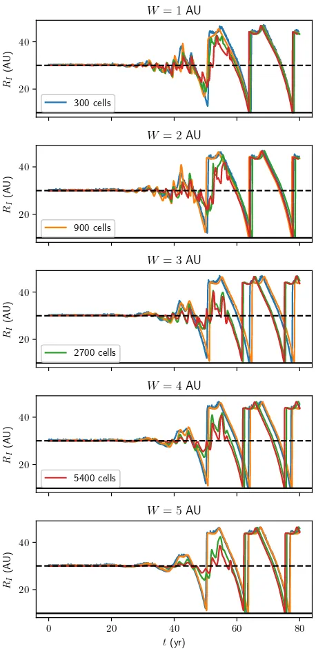
Fig.8shows the ionization front radius as a function of time for the same simulations when we self-consistently up-date the ionization state. All simulations still become unsta-ble after some time, with the instability still being seeded by numerical noise. Since the noise depends on the resolution, the instability is seeded differently for different resolutions, and we do not obtain a converged result.

To seed the instability, we use the output of the set up runs shown in Fig.7and add a small gaussian-like density perturbation filter φ(r) to the density, such that ρ′

(r) =

20 40

RI

(A

U

)

W = 1AU

300 cells

20 40

RI

(A

U

)

W = 2AU

900 cells

20 40

RI

(A

U

)

W = 3AU

2700 cells

20 40

RI

(A

U

)

W = 4AU

5400 cells

0 20 40 60 80

t(yr)

20 40

RI

(A

U

)

W = 5AU

Figure 8.Ionization front radius as a function of time for simula-tions with a smooth transition from ionized to neutral region, self-consistent ionization, and a numerically seeded instability. The full lines show simulation results for different spatial resolutions, as indicated in the legend. The dashed horizontal line shows the initial ionization front radius, the full horizontal line shows the radius of the inner outflow boundary.

φ(r)ρ(r):

φ(r) =   

 

1 +ρp 1−6u2+ 6u3

u < 1₂, 1 + 2ρp(1−u)3 1

2 ≤u <1,

1 1≤u,

(47)

10−17

10−16

ρ

(g

cm

−

3)

t= 0.0 yr t= 6.5 yr t= 8.5 yr t= 13.0 yr t= 18.0 yr

20 40 60 80 100

r(AU)

−50 −40 −30 −20

v

(k

m

s

−

1)

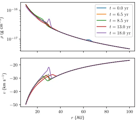
Figure 9.Density and velocity profile for the stability test run withρp= 0.1, at 5 significant times throughout the simulation, as indicated in the legend. The dashed line shows the analytic two temperature solution for the same parameters.

cubic spline kernel commonly used in SPH codes (see e.g.

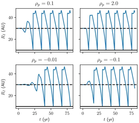
Springel 2005). We will user0= 65 AU andh= 5 AU. We will choose 4 different amplitudes for the perturbation to test the various scenarios derived above:ρp= 0.1, ρp= 2, ρp =−0.1 andρp =−0.01. These correspond respectively to a small positive seed that should cause an ionization front movement slower than the accretion velocity, a large posi-tive seed that should cause the immediate collapse of the ionization front, a negative seed that should initially cause an expansion of the ionization front followed by a collapse, and a negative seed that should cause a number of oscilla-tions.

Fig. 9shows the time evolution of a simulation with a small positive seed perturbation. The perturbation initially moves inwards with the accretion flow until it reaches the ionization front. Once it arrives there, it causes an increase in the density inside the ionization region, which causes the ionization front radius to shrink according to equation (37). The density enhancement continues to move inwards with the accretion flow, and for a while the ionization front moves inwards as well. The region outside the ionization front ra-dius in the meantime adjusts to the lower pressure and set-tles into a neutral Bondi accretion, with an overall lower density.

When the initial perturbation reaches the inner outflow boundary, the mass inside the perturbation is effectively lost from the system, causing the density inside the ionized re-gion to go down again, and subsequently the ionization front radius to expand again. However, since the density inside the original ionization front radius partially settled into a neu-tral Bondi profile, the overall density inside the ionized re-gion will be lower than in the steady state two temperature solution, and the new ionization front radius will expand beyond the original ionization front radius. This is not a steady state solution anymore, so the ionization front radius

20 40 60

RI

(A

U

)

No smoothing

300 cells

20 40 60

RI

(A

U

)

W= 1_AU

900 cells

20 40 60

RI

(A

U

)

W= 2_AU

2700 cells

20 40 60

RI

(A

U

)

W= 3_AU

5400 cells

t(yr)

20 40 60

RI

(A

U

)

W= 4_AU

0 20 40 60 80

20 40 60

RI

(A

U

)

W= 5_AU

20 40

RI

(A

U

)

ρp= 0_.1 _ρp= 2_.0

0 25 50 75 t(yr)

20 40

RI

(A

U

)

ρp=₋0_.01

0 25 50 75 t(yr)

ρp=₋0_.1

Figure 11.Ionization radius as a function of time for simulations with 4 different values for the perturbation amplitudeρp, as in-dicated above each panel. All simulations are based on the same initial condition with a smooth ionization transition of 5 AU and use a resolution of 2700 cells. The dashed black lines show the initial ionisation radius, while the full black lines correspond to the radius of the inner outflow boundary.

will consequently shrink again as the inner density adapts to the ionization again. During that process, a large peak in density builds up around the ionization front radius, which in combination with the ionization front evolution (equation (37) leads to a runaway collapse of the ionization front to-wards the mask. Once this peak reaches the inner outflow boundary, the situation is reset again, and the whole process repeats itself.

Fig. 10shows the evolution of the ionization front ra-dius as a function of time for the simulations with a negative seed perturbation with ρp =−0.1. We clearly see how the repeated runaway collapse of the ionization front leads to a periodic oscillation of the ionization front radius with a period of∼10 yr, roughly consistent with the free fall time of the system. It is clear that the combination of a smooth transition that damps small scale noise and the seeding of the instability with a well defined perturbation allow us to achieve numerical convergence for the high resolution simu-lations. This in principle should allow us to use this test as a benchmark for this type of instability. Note that the conver-gence is better for initial conditions with a larger transition region from fully ionized to fully neutral. For what follows, we will hence limit ourselves to simulations with an ioniza-tion transiioniza-tion of 5 AU and a resoluioniza-tion of 2700 cells.

Note that the expanding ionization front at the end of each oscillation moves relatively fast, so that we cannot guarantee that the dynamical time for this expansion is sig-nificantly larger than the recombination time; a main as-sumption for our ionization treatment. However, the overall density inside the central region is low enough to guaran-tee the build up of a new ionization front at the expected radius in a time that is short enough not to significantly al-ter our dynamics, and we can hence still assume our results

are qualitatively correct, albeit with a slightly longer oscil-lation period. We confirmed this using a time dependent Monte Carlo radiative transfer simulation. Similarly, mov-ing the inner outflow boundary to smaller radii will lead to a small increase in oscillation period, but will not change the qualitative behaviour, as we still expect accreted material at small enough radii to be lost from our system of interest.

Fig.11shows the time evolution of the ionization radius for the 4 different scenarios discussed in2.4. In the case of a positive density perturbation, the ionization front initially collapses. If the bump is small, the ionization front does not move at the same speed as the bump, and the collapse halts when the bump moves accross the inner outflow boundary. If the bump is large enough, the ionization front moves along with the bump and both collapse onto the inner outflow boundary.

For a negative density bump, the ionization front ini-tially expands until the density bump is accreted accross the inner boundary. At this point, the expanded ionization re-gion will start to contract again. For a large negative bump, this immediately leads to a collapse of the ionization front. For smaller bumps, the collapse is only partial and leads to an oscillation of the ionization front with an amplitude that increases over time.

In all cases, the initial perturbation eventually evolves into a periodic oscillation of the ionization front, i.e. all sce-narios naturally evolve into the case where the ionization front movement becomes coupled to the movement of the density perturbation.

These simulations hence confirm the semi-analytic model we derived before.

3.1.6 TORUS comparison

To investigate the impact of our approximations on the re-sult of the 1D models, we reran our 1D test with the radi-ation hydrodynamics codetorus_{(Harries 2000), using the} “detailed” model as described inHaworth et al.(2015). This includes polychromatic radiation transport, diffuse field ra-diation (i.e. not the on-the-spot approximation) as well as helium, metals and the associated line cooling in the thermal balance. In these calculations a hydrodynamics-only calcu-lation is run until a steady state is reached. The medium is the fully ionized, which lowers the optical depth and hence speeds up the convergence of the first photoionization equi-librium calculation. Subsequently, photoionization and hy-drodynamics steps are performed iteratively to follow the RHD evolution. The ionizing luminosity of the source was tuned to approximately reproduce the same ionization front radius as in the models above.

30 40 50 60 70

t(yr) 10

15 20 25 30

RI

(A

U

)

Figure 12. Ionization front as a function of time for a self-consistent RHD simulation of a single ionizing source within an initially stable neutral Bondi profile, simulated withtorus. The black lines represent the initial ionisation front radius (dashed) and the mask radius (full).

3.2 3D simulation

The presence of a 1D instability has important implications for 3D RHD simulations of spherically symmetric Bondi ac-cretion. If spherical symmetry is not explicitly imposed on the radiation field or on the coupling between radiation field and hydrodynamics, then the instability will be seeded dif-ferently in different directions. Once initial asymetries have been seeded, the problem is no longer spherically symmetric and true 3D effects will govern the hydrodynamical evolu-tion.

We explore these effects by running the same Bondi set up described above in a full 3D RHD simula-tion using the Monte Carlo RHD code CMacIonize (Vandenbroucke & Wood 2018). Since we are not interested in the detailed results, we limit ourselves to low resolu-tion simularesolu-tions and do not explicitly check for convergence. More realistic simulations will be subject of future studies. We run two simulations with different grids used to dis-cretize the fluid. Both simulations follow a fluid in a box of 100 AU×100 AU×100 AU with inflow boundary condi-tions and a point mass (and ionization source) at the centre. Just as for the 1D simulations, a central sphere with radius 10 AU is masked out. The mass, initial ionization radius, neutral Bondi density, neutral gas temperature and pressure contrast are set as before.

A first set up uses a regular Cartesian grid of 128×

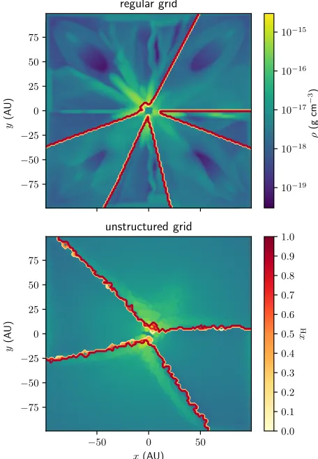
128×128 cells. To compute the ionization front position, we use 107 Monte Carlo photon packets and 10 iterations. Ini-tial instabilities will be seeded by two mechanisms: Poisson noise inherent to the Monte Carlo method, and discretiza-tion error due to the low resoludiscretiza-tion grid used. The latter will have a strong dependence on specific grid directions (e.g. the coordinate axis directions and diagonals), and from the top panel of Fig.13it is clear that they constitute the dominant seeding mechanism, resulting in a very symmetrical, yet no longer spherically symmetric ionization region.

The higher pressure in the directions with a larger ion-ization radius will cause a tangential force that evacuates these regions and pushes material into directions that are

−75

−50

−25 0 25 50 75

y

(A

U

)

regular grid

−50 0 50

x(AU)

−75

−50

−25 0 25 50 75

y

(A

U

)

unstructured grid

10−19

10−18

10−17

10−16

10−15

ρ

(g

cm

−

3)

0.0 0.1 0.2 0.3 0.4 0.5 0_.6 0_.7 0.8 0.9 1.0

xH

Figure 13.Density slice atz= 0 for a 3D Bondi accretion sim-ulation with self-consistent photoionization and using a regular Cartesian grid of 128×128×128 cells (top) and an unstruc-tured Voronoi grid with 100,000 cells (bottom). Both simulations were started from the same initial density profile and evolved self-consistently untilt= 20 yr.

still neutral, reenforcing the differences between both re-gions. While some directions with larger ionization radii still periodically collapse due to the radial instability, the direc-tions with a smaller ionization radius actually remain stable. At later times, the ionization region has a chaotic, asymmet-ric shape, while the density field shows clear signs of grid symmetries.

To eliminate the effect of Cartesian grid symmetries, we run the same simulation using an unstructured Voronoi grid consisting of 100,000 cells, using 106 photon packets for 10 iterations. This is the same grid structure used to run CMacIonizeas a moving-mesh code, but without actually moving the mesh in between time steps (since this would be very complicated for a 3D problem with spherical accretion). In this case, the results look less artificial (see bottom panel of Fig. 13), but the qualitative interpretation is the same: the combination of the 1D instability and 3D effects will cause the ionization front to break up into a non-spherically symmetric structure, and the ionization front will stabilize in some directions.

per-fectly spherically symmetric manner, 3D simulations will never result in a perfectly symmetric ionization region, irre-spective of any additional 3D effects that could be included in these simulations. This is valuable background knowledge for the interpretation of future 3D studies of Bondi accretion that will include rotation, and a general limitation for RHD codes in studying problems that involve both accretion and photoionization.

4 CONCLUSION

In this work, we studied the stability of spherically sym-metric ionized Bondi accretion flows around young stellar objects. We derived an anlytic expression for a two tempera-ture steady state solution in which an R type ionization front with a size of the order of 10 AU is trapped in the highly supersonic accreting flow, consistent with the predictions of

Keto (2002, 2003). We were able to accurately reproduce this analytic profile in a constrained 1D RHD simulation.

However, we also showed that this steady state solu-tion is only marginally stable if ionizasolu-tion is treated self-consistently, leading to a collapse of the ionization front un-der small perturbations in density or ionizing luminosity. We were able to confirm our semi-analytic model of this insta-bility using 1D RHD simulations, and were able to obtain spatially converged results by introducing a noise suppress-ing transition layer and a seeded instability.

Both the constrained simulations that lead to the two temperature steady state solution and the converged simu-lations of the instability could serve as benchmark problems for 1D RHD codes.

Finally, we showed that the existence of a 1D instabil-ity has profound implications for 3D simulations of ionized accretion flows when the radiation field is not treated in a perfectly spherically symmetric manner. The instability makes it impossible to retain spherical symmetry, and will amplify grid symmetries.

ACKNOWLEDGEMENTS

We want to thank the anonymous referee for constructive and insightful comments regarding the convergence of our simulations. BV and KW acknowledge support from STFC grant ST/M001296/1. NS would like to thank CAPES for graduate research funding. KL acknowledges support from the Carnegie Trust. DFG thanks the Brazilian agencies FAPESP (no. 2013/10559-3) and CNPq (no. 311128/2017-3) for financial support. TJH is funded by an Imperial College London Junior Research Fellowship.

REFERENCES

Beltr´an M. T., de Wit W. J., 2016,A&ARv,24, 6

Bondi H., 1952,MNRAS,112, 195

Churchwell E., 2002,ARA&A,40, 27

Cranmer S. R., 2004,American Journal of Physics,72, 1397

Harries T. J., 2000,MNRAS,315, 722

Haworth T. J., Harries T. J., Acreman D. M., Bisbas T. G., 2015,

MNRAS,453, 2277

Hopkins P. F., 2015,MNRAS,450, 53

Ilee J. D., Cyganowski C. J., Nazari P., Hunter T. R., Brogan C. L., Forgan D. H., Zhang Q., 2016,MNRAS,462, 4386

Keto E., 2002,ApJ,580, 980

Keto E., 2003,ApJ,599, 1196

Kuiper R., Hosokawa T., 2018,A&A,616, A101

Mestel L., 1954,MNRAS,114, 437

Osterbrock D. E., Ferland G. J., 2006, Astrophysics of gaseous nebulae and active galactic nuclei. University Science Books, Sausalito, CA

Springel V., 2005,MNRAS,364, 1105

Springel V., 2010,MNRAS,401, 791

Sternberg A., Hoffmann T. L., Pauldrach A. W. A., 2003,ApJ,

599, 1333

Toro E. F., 2009, Riemann Solvers and Numerical Methods for Fluid Dynamics, 3rd edn. Springer-Verlag

Vandenbroucke B., Wood K., 2018,Astronomy and Computing,

23, 40

APPENDIX A: ANALYSIS OF STRONG AND WEAK R TYPE SOLUTIONS

Here we perform a detailed analysis of equation (15) for the case of an R type front, withvn(RI)<−vR. We begin by rewriting the equation in terms of the dimensionless vari-ablesx=−vn(RI)/Cs,iandA=Cs,n/Cs,i:

Γ(x, A) = 1 2

x2+A2±p(x2_+A2₎2_−4x2_{. (A1)}

Note thatA=p

1/Pc<1. To get a real solution, we require

x >1 +p1−A2_{, (A2)}

and hence the neutral region is supersonic. For the critical valuexc= 1 +√1−A2_,

Γc(A) = 1 + p

1−A2_{=xc>1, (A3)} which implies vi(RI) = −Cs,i > vn(RI). We now explore how the value of Γ changes forx > xcin the case of a strong and a weak R type front.

The first derivatives of Γ(x, A) are

∂Γ(x, A)

∂x =x±

(A2+x2−2)x p

(x2_+A2₎2_−4x2, (A4) ∂Γ(x, A)

∂A =A±

(A2_+x2_)A p

(x2_+A2₎2_−4x2. (A5) Forx > xc and 0< A <1, these derivatives have no real roots, which means Γ(x, A) is monotonous in these regions. Furthermore, we have that∂Γ(x, A)/∂x→ ± ∞forx→xc, which means that Γ>Γc for a strong R front, and Γ<Γc for a weak front.

For the weak front, we find (note the signs):

Γ = vn(RI)

vi(RI) <Γc=xc= vR Cs,i <

−vn(RI)

Cs,i , (A6)

or

vi(RI)<−Cs,i, (A7)

which means that the ionized region is always supersonic. For a strong R type front the condition Γ > Γc does not impose similar restrictions, so that a strong front can be subsonic or supersonic.

supersonic or subsonic. From our analysis, it follows that a weakR type front, defined as the front with the smaller jump in density and velocity across the ionization front, isalways supersonic, and is the only front expected to exist in nature.

Thestrong front, defined as the front with a larger jump in

density and velocity across the ionization front, can be either supersonic or subsonic. For the critical casevn(RI) =−vR, the strong and weak front are the same, and the ionized velocity is the ionized sound speed.