Comparison between Theoretical and Experimental Radial Electron Temperature Profiles in a Low Density Weakly Ionized Plasma

http://www.scirp.org/journal/jmp ISSN Online: 2153-120X ISSN Print: 2153-1196

DOI: 10.4236/jmp.2019.107050 Jun. 14, 2019 699 Journal of Modern Physics

Comparison between Theoretical and

Experimental Radial Electron Temperature

Profiles in a Low Density Weakly Ionized

Plasma

Ahmed Rida Galaly1,2*, Guido Van Oost3,4,5

1_{Department of Physics, Faculty of Science, Beni-Suef University, Beni Suef, Egypt}

2_{Department of Engineering Science, Faculty of Community, Umm Al_Qura University, Mecca, Mecca Province, KSA} 3_{Department of Applied Physics, Ghent University, Technicum B4, Ghent, Belgium}

4_{National Research Nuclear University “MEPHI”, Moscow, Russia}

5_{National Research University “Moscow Power Engineering Institute”, Moscow, Russia}

Abstract

Experimental and theoretical studies of the radial distribution function of the electron temperature (RDFT) in a low-density plasma and weakly ionized gas for the abnormal glow region are presented. Experimentally, the electron temperatures and densities are measured by a Langmuir probe moved radially from the center to the edge of the cathode electrode for helium gas at differ-ent pressures in the low-pressure glow discharge. The comparison of the final experimental data for the radial distribution of electron temperatures and densities for different low pressures ranging from 0.2 to 1.2 torr, with the fi-nal proved equation of RDFT confirms that the electron temperatures decrease with increasing product of radial distance and gas pressures, show-ing a radial decrement dependence of the electron temperature from the cen-ter to the edge of the electrode. This is attributed to the increase of the num-ber of electron-atom collisions at higher gas pressures and consequently of the rate of ionization. For the axial distance (L) from the tip of the probe to cathode electrode and the cathode electrode radius (R), a theoretical and ex-perimental comparison for the two conditions L < R and L > R, for both cases the produced plasma temperatures decrease and densities increase. It is con-cluded that the RDFT accurately shows a dramatic decrease for L < R by 60% less than RDFT values for L > R similar as for conditions of magnetized and unmagnetized effect for DC plasma. This means that the rate of plasma loss by diffusion decreased for L < R, agrees well with the applied of magnetic

How to cite this paper: Galaly, A.R. and Van Oost, G. (2019) Comparison between Theoretical and Experimental Radial Elec-tron Temperature Profiles in a Low Density Weakly Ionized Plasma. Journal of Modern Physics, 10, 699-716.

https://doi.org/10.4236/jmp.2019.107050

Received: May 15, 2019 Accepted: June 11, 2019 Published: June 14, 2019

Copyright © 2019 by author(s) and Scientific Research Publishing Inc. This work is licensed under the Creative Commons Attribution International License (CC BY 4.0).

http://creativecommons.org/licenses/by/4.0/

DOI: 10.4236/jmp.2019.107050 700 Journal of Modern Physics

field behavior.

Keywords

Radial Distribution, Electron Temperature, Ambipolar Diffusion, Low Pressure, Weakly Ionized Plasma

1. Introduction

Plasma is the fourth state of matter, considered to be a quasi-neutral medium. However, when a diagnostic such as probe (a small metallic electrode) is inserted into a weakly ionized plasma, a very thin sheath is formed around the conduct-ing surface of the probe due to the redistribution of charges. The amplitude and the polarity of the probe potential control the motion of electrons and ions near the probe. When the probe potential is sufficiently negative, only the ions can reach the probe surface. The probe current is thus equal to the ion random cur-rent (Iri) [1][2][3].

Ambipolar diffusion is the most important process taking place within a weakly ionized plasma and considered as a vital process for the distribution of the plasma parameters. Assuming a Maxwellian velocity distribution [4], the plasma parameters especially electron temperature and electron density can be determined from the current-voltage characteristic curves of the probe [5]. Dif-fusion phenomenaoccur in a plasma when a spatial gradient of the charged spe-cies is present [6]. Furthermore, it is caused by the differently charged species having different diffusivities, hence there is a loss of neutrality [7] due to plasma rapidly diffusion for some of charged species more than the others. Furthermore, a minor loss of neutrality, however, induces an ambipolar electric field which, if the Debye length is sufficiently small, slows down the fast-diffusing species and speeds up the slow-diffusing species in such a way that the plasma remains qua-si-neutral [8].

The experimental and numerical radial distribution of electron temperature and density from the axis of the tube up to the tube wall have been amply inves-tigated [9] [10], but not the theoretical derivation in terms of the effect of Schottky condition and ambipolar diffusion due to the recurrence relation of the Bessel condition.

DOI:10.4236/jmp.2019.107050 701 Journal of Modern Physics

2. Experimental Study

2.1. Experimental Set-Up

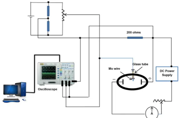
Figure 1 shows the experimental setup of DC (cold cathode) magnetron sput-tering unit to generate a glow discharge in a glass tube between two circular, pa-rallel and movable metallic discs acting as electrodes. Two papa-rallel electrodes made of aluminum, are enclosed in the discharge cell, one of the two electrodes is grounded represented cathode electrode and the other is movable to change the axial distance represented the anode electrode, where the axial distance (L) between tip of the probe and the cathode electrode, 5 cm and with 3 cm in radius (R) taking into account that we will deal with two conditions R > L and R < L. The discharge unit is evacuated using a rotary pump to a base pressure of 7 mtorr. A pressure gauge is connected to the discharge tube to measure the inside gas pressure. A stationary DC-glow discharge was generated between two both electrodes, for different parameters as shown in Table 1.

Figure 1 also shows the schematic diagram of the spherical single Langmuir probe circuit. The probe made of molybdenum wire (diameter 3.0-mm and length 0.5 mm) and the tip of a probe is inside the glow discharge plasma. The single probe (between the cathode fixed at the ground potential, and the anode) move axially to measure the axial potential distribution between the two trodes. Also, it moves radially from the center to the edge of the cathode elec-trode, and a potential VP is applied to the probe.

2.2. Experimental Study of Axial Potential and Electric Field Distribution Measurements

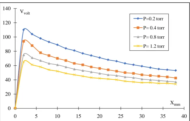
The potential distribution was measured at discharge currents of 10 mA and gas pressure of (0.2 - 1.2 torr) for He as shown in Figure 2, shows that the potential

Figure 1. Schematic diagram of the experimental setup and the single Langmuir probe

DOI: 10.4236/jmp.2019.107050 702 Journal of Modern Physics

Figure 2. Axial potential distribution at constant current (I = 10 mA).

Table 1. Shows the values of operating parameters.

Parameters Values

Discharge Current (Ia) 4 - 30 mA

Gas Pressure (P) 0.1 - 1.5 torr Discharge Voltage (Va) 200 - 1200 V DC

Current Density 2 - 15 mA/m2

Working Gas He

distribution can be divided into three regions. In region I (AB) (cathode fall), the potential increases sharply within a small discharge length. Whenever, gas breakdown takes place in the tube, a rapid growth in the rate of ionization, near the cathode is detected. Meanwhile the electrons transfer in the electric field much more faster than positive ions (due to their masses), electrons are swept rapidly towards the anode leaving a dense positive space charge near the cathode. Thus, the electric field is distorted and most of the applied potential is dropped across a narrow space in front of the cathode. Region II (BC) (negative glow) in-dicates that the potential decreases slightly and hence the electric field will be weak, since this region contains many free electrons. In region III (CD) (positive column), the potential distribution is nearly constant and linear since the posi-tive and negaposi-tive carriers densities are closely, equal. The posiposi-tive column can be extended to any length to fill the remaining space between the end of the nega-tive glow and the anode.

Values of the electric field distribution are obtained by differentiating the measured potential distribution of Figure 2. Figure 3 and Figure 4 show the electric field distribution for He discharge. In the cathode fall region at edge and center, high electric field is observed which is decreased sharply away from the

0 20 40 60 80 100 120 140

0 5 10 15 20 25 30 35 40

V_volt

X_mm

DOI:10.4236/jmp.2019.107050 703 Journal of Modern Physics

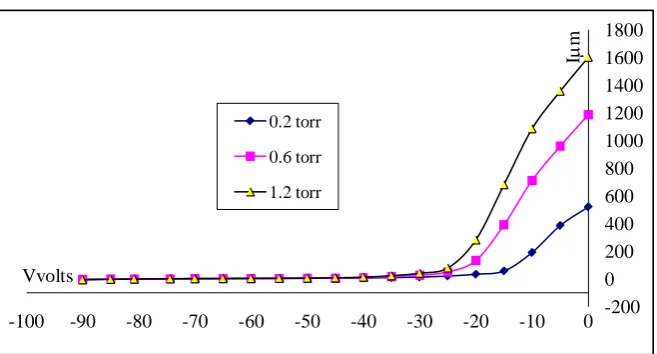
Figure 3. I-V curves of the single probe for cathode fall region at different He pressures at the edge.

Figure 4. Measured I-V curves of the single probe for cathode fall region at different He pressures at the center.

cathode. This is related to the intense positive space charge which lies in front of the cathode. This acts as an accelerator for the electrons towards anode. Thus, the electrons emitted from the cathode are then accelerated away, until they reach the negative glow region where the electric field becomes weak (zero and sometimes it reaches a negative value). In this region, the gained kinetic energy of the electrons is dissipated in collisions with the atoms of the gas and thus secondary electrons would be produced. In the positive column region constant and linear electric field is needed to maintain discharge along the large length of the column which is required to carry the discharge current.

2.3. Experimental Study of Radial Dependence of the Electron Temperature

The region investigated in the present work is the abnormal region. The radial

-50 0 50 100 150 200 250 300 350

-90 -80 -70 -60 -50 -40 -30 -20 -10 0

I

µ

m

V volts

0.2 torr

0.6 torr

1.2 torr

-200 0 200 400 600 800 1000 1200 1400 1600 1800

-100 -90 -80 -70 -60 -50 -40 -30 -20 -10 0

I

µ

m

Vvolts

0.2 torr

0.6 torr

DOI: 10.4236/jmp.2019.107050 704 Journal of Modern Physics

dependence of the electron temperature in low-density plasma at edge and cen-ter of the cathode electrode has been studied for different He pressures.

The plasma parameters like the electron temperature and electron density can be determined from the current-voltage (I-V) characteristic curve of the single Langmuir probe, based on the theory and the fundamental technique discussed in detail in many articles [10][11].

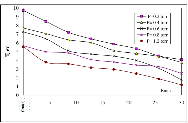
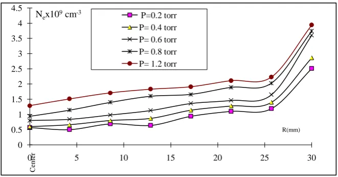
Figure 3 and Figure 4 show I-V characteristic curves of the single probe at different He pressures at edge and center of the cathode electrode for the ab-normal glow region [12]. The probe was moved to investigate the radial distri-bution from the center to the edge of the cathode, in the direction perpendicular to the direction of the electric field lines. Figure 5 and Figure 6 show the radial temperatures and densities distributions at different pressures from center to the edge. Te is decreased and ne increased due to the general trend that values of Te and ne are inversely proportional [13].

Increasing the helium working pressures from 0.2 to 1.2 torr, the temperature Te decreases at the center from 9.7 eV to 5.5 eV and at the edge from 4.1 to 1.15 eV. Values of densities ne increased at center ne from 0.6 × 109 cm−3 to 1.3 × 109 cm−3 _{and at the edge from 2.5 to 3.95 × 10}9 _cm−3_.

3. Theoretical Consideration of the Radial Dependence of

the Electron Temperature

Conductivity at the tube axis, and charge density of plasma according to the fol-lowing expression [14][15]

1

s a e

D D µ ρ

σ

= _ − _

  (1)

where Da is the ambipolar diffusion coefficient as follows: The flow of ions and electrons are the same, hence

Figure 5. The Experimental radial temperature distribution of abnormal region for

he-lium at different pressures.

0 1 2 3 4 5 6 7 8 9 10

0 5 10 15 20 25 30

Te

ev

Rmm

P=0.2 torr P= 0.4 torr P= 0.6 torr P= 0.8 torr P= 1.2 torr

C

en

te

DOI:10.4236/jmp.2019.107050 705 Journal of Modern Physics

Figure 6. Measured radial density distribution of abnormal region for helium at different pressures.

i e

Γ = Γ = Γ

(Congruence approximation). If there is no external electric field, the fluxes of ions and electrons (drift-diffusion model) can be expressed as:

i D ni i µin Ei D

Γ = − ∇ +

e De ne µe en ED

Γ = − ∇ +

where ED follows Poisson’s equation. If we multiply the first equation by µene

and the second one by µi in and then subtract them, we get:

ini e e en i e en D ni i e en in Ei D in Di e ne ini e en ED

µ Γ −µ Γ =µ ∇ −µ µ −µ ∇ +µ µ

Since Γ = Γ = Γi e, the terms with ED cancel each other out and using ne = ni,

the expression for the flow of particles becomes:

(

)

i e

i D

n

Dµ µ

µ µ

Γ

− −

∇ −

=

With the ambipolar diffusion coefficient being

e e

a

e

D D

D µ µ

µ+₊−µ+ −

= ₍₂₎

and ρ _{is the charge density in the plasma given by:}

[

]

e n n

ρ= +− (3)

and σ is the conductivity at the tube axis given by:

[

]

e n n

σ= µ+ +−µ (4)

Considering that diffusion coefficient D given by:

2 m s kT D

mν

= (5)

where µε,+ are the mobility of electrons (e) and ions (+), kT (ev) is the particle

temperature, ν _{is the collision frequency between electrons and neutral atoms}

in Hz. By substituting with Equations (2, 3 and 4) into Equation (1), then we get

0 0.5 1 1.5 2 2.5 3 3.5 4 4.5

0 5 10 15 20 25 30

Nex109cm-3

R(mm)

P=0.2 torr P= 0.4 torr P= 0.6 torr P= 0.8 torr P= 1.2 torr

C

en

te

DOI: 10.4236/jmp.2019.107050 706 Journal of Modern Physics 1

e e e

s e

e e e

D D n n

D

n n

µ µ

µ

µ µ µ µ

+ + + + + +   − − = _ − _ −  

− (6)

But by substituting by the Einstein relation [16][17]:

q D

kT

µ=   (7)

into Equation (6) by the value of D, then we get

(

)

e e e e

s e

e e e

KT KT n n

D

q n n

µ µ µ µ _µ

µ µ µ µ

+ + + + + + +   − − = _ − − 

− _ (8)

or

(

)

(

)

e e e e e e

s

e e

e

e

KT KT n n n n

D

e n n

µ µ µ µ µ µ

µ µ µ µ

+ + + + + + + + −  − − +  = _ − 

− _ (9)

Neglecting kT+, where kTekT+ finally results in

Then

( )

(

)

s

e e e

n kT

D

e n n

µ µ µ µ

µ µ µ µ

+ + +

+ + +

 − 

=

− _ − _ (10)

( )

e e

s

e e

n kT

D

e n n

µ µ µ µ + + + +   = _{ } −   Then e e s e e kT D n e n µ µ µ µ + + +       =  ₋      (11) or 1 e e s e e kT D n e n µ µ µ+ +

      =  ₋      (12)

Substituting e e e e m

µ ν

= and i

i i

e m

µ ν

= from Equations (5) and (7) into

Eq-uation (12) results in

DOI:10.4236/jmp.2019.107050 707 Journal of Modern Physics 1

1 e e

S e

i i e

e e m D kT m n m n ν ν ν +       =  ₋      (14) or S e

e e i i e

n

D kT

mν n mνn

+

+

 

= _{ }

−

  (15)

2

S e

i i e

e e i i

D kT

m n

m

n

ν _{ν ν} ν

+ =

−

(16)

Experimentally, due to the diffusion process during plasma formation an in-teresting process occur in the plasma formation stage of the basil discharge. Theoretically, basil discharge process related with the recurrence relation for Bessel condition as shown in appendix A, where from the recurrence relation for the Bessel condition, the Schottky condition can be derived and proofed [18][19] stating that:

3.1. In the Case of L (Axial Distance) > R (Radial Distance) 2 2.405 S i D R ν  

= _ _ (17)

A proof of the Schottky condition will be discussed briefly by two methods in Appendix A, where (R cm) represents the radial distance from the center to the edge through the cathode electrode measured by the Langmuir probe moved ra-dially, and by substituting Equation (17) into (16), then

2 2

2.4

e

i i e e e i

kT R m n m n ν ν ν +  _{ =}  

  ₋ (18)

Substituting the following equation into Equation (18)

-

-e Nn Qe n e n

ν = υ _(19a)

(

)

-2

3.55 10 e

e e n

e kT P Q

m

ν = × _ _

  (19b)

(

)

-2

3.55 10 i

i i n

i kT P Q

m

ν = × _ _

  (19c)

where P in torr, Qe n- and Qi n- are the cross sections of electron-neutral and

ion-neutral collisions, respectively results in

(

)

(

)

2

1 2 1 2

2

2 2

16 16

2.4 _{2 2 2}

3.55 10 3.55 10

e

e i e i

e i e i i

e i i

kT R

kT kT n kT

m P Q Q m P Q

m m n+ m

DOI: 10.4236/jmp.2019.107050 708 Journal of Modern Physics then

(

)

(

)

2.4 _{4 2}

3.55 10 3.55 10

e i e i

i e i

i e i e

RP

m kT n kT

Q Q Q

m kT n+ m kT

 _{ =}   _{ }   _  _{× −} _×                 (21)

But from [20][21]

( )

≅ (22a)

Then substituting (7) into (22a) gives

2 1 7.64 i i e kT m kT      

≅ (22b)

Moreover, substituting (22b), i 2000 e m

m ≅ and

2 10 i e ν ν −

≅ _{into (21) gives}

(

)

(

)

2

1 2 2

2 2

16 16

1

2.4 _{4 2}

7.64 i e i 3.55 10 e 3.55 10 7.64 i i

i e i

e e e e

RP

kT m kT n kT kT

Q Q Q

kT kT n+ kT kT

 _{ =}   _{   }   _{    } _{  } ×  − × _{ }                 (23)

( )

(

)

(

)

1 2 2

2 2

16 16

2.4

4 2

7.64 i e i 3.55 10 e 3.55 10 7.64 i i

i e i

e e e e

RP

kT m kT n kT kT

Q Q Q

kT kT n+ kT kT

= _{  }   _{ } _{  } ×  − × _{ }               _   (24)

Substituting the values of the cross sections, masses of ions and electrons into (24) gives

( )

(

) (

)( )

2 2

1 2 2

2

2.4

3.55 7.64 2 i e i e7.64 i i

e e e e

RP

kT m kT n kT kT

kT kT n+ kT kT

  _{ }     =      _  _ −       _   _         (25) or

( )

(

) (

)( )

3 2 3 2

2 1 2

2.4

3.55 7.64 2 i 7.64 e i

e

e e

RP

kT n kT

m

kT n+ kT

=     _   _ −         _   _ (26) Then finally 1 2

3 4 3 2

1 2 1 0.1729

7.64

i e i

e

e e

RP

kT n kT

m

kT n+ kT

=     _{ − }   _{ }  _{ } _{ }     (27)

DOI:10.4236/jmp.2019.107050 709 Journal of Modern Physics

and Figure 5 respectively, into the Equation (27), taking into account that

e i

T T (Ti=0.1Te), 2000

e

i m

m ≅ [22] and for the spherical probe, the ion

density is given by [23]:

1 2

0.6 P

e

i kT I

n A

m

+ +

 

= _{ }

  (28)

Knowing Te, (Ap =4πrp2) area of spherical probe) and calculating positive ion

current I+ from the I-V characteristic curve of the spherical single probe [24], n+ can be determined.

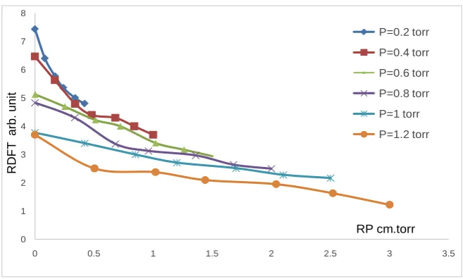
Figure 7 shows the radial distribution of the electron temperature (RDFT) theoretically using Equation (27), in the abnormal cathode fall region from the center to the edge of the electrode as a function of He as an inert gas. The RDFT from the theoretical method presented above accurately shows a dramatic radial reduction of the electron temperature for any region (cathode fall or negative glow or positive column) and for any applied pressure. Furthermore, the decre-ments of Te at the edge of the electrode are more pronounced at the center due to edge effect [25].

3.2. In the Case of L (Axial Distance)< R (Radial Distance)

2 2

2.405 π

S

i

D R L

ν

   

=_{ } +_{ }

    (29)

and by substituting Equation (29) into (16), then

2 2

2

2.4 π _i

e

i e

e e i

kT

R L

m n

m

n

ν ν ν

+

  ₊  ₌

   

    ₋ (30)

Substituting by Equations (19a, b and c) into Equation (30), respectively re-sults in

Figure 7. Theoretical radial distribution of the electron temperature (RDFT).

0 1 2 3 4 5 6 7 8

0 0.5 1 1.5 2 2.5 3 3.5

R

D

F

T

ar

b.

uni

t

RP cm.torr

P=0.2 torr

P=0.4 torr

P=0.6 torr

P=0.8 torr

P=1 torr

DOI: 10.4236/jmp.2019.107050 710 Journal of Modern Physics

(

)

(

)

2 2

1 2 1 2

2

2 2

16 16

2.4 π _{2 2 2}

3.55 10 3.55 10

e

e i e i

e i e i i

e i i

kT

R L

kT kT n kT

m P Q Q m P Q

m m n₊ m

  ₊  ₌     _{ }          _{ }        × − _ × _              (31) then

(

)

(

)

2.4 π _{4 2}

3.55 10 3.55 10

e i e i

i e i

i e i e

R L

m kT n kT

Q Q Q

m kT n+ m kT

  ₊  ₌     _{ }     _  _    × − ×              (32)

Substitution from (22a and b) into (32) gives

(

)

(

)

2 2

1 2 2

2 2

16 16

1

2.4 π _{4 2}

7.64 i e i 3.55 10 e 3.55 10 7.64 i i

i e i

e e e e

RP L

kT m kT n kT kT

Q Q Q

kT kT n+ kT kT

  ₊  ₌     _{   }     _{      } _{  } ×  − × _{   }              (33)

( )

(

)

(

)

1 2 2

2 2 16 16 2.4 2.4 π 4 2

7.64 i e i 3.55 10 e 3.55 10 7.64 i i

i e i

e e e e

L RP

kT m kT n kT kT

Q Q Q

kT kT n₊ kT kT

  = _{ } _{  }   _{   }   _{  } ×  − × _{   }              − (34)

Substituting the values of the cross sections, masses of ions and electrons into (34) gives finally

2

3 2 3 2

1 2 0.0299

5.76 π 7.64

i e i

e

e e

L RP

kT n kT

m

kT n₊ kT

                     _{   }    = − _{ }     −     _{  }  (35)

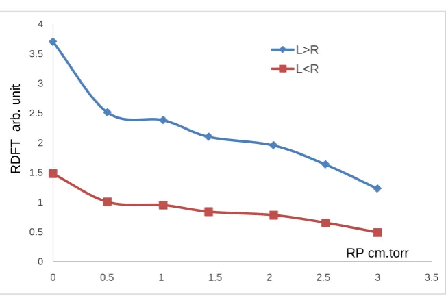
For 1.2 torr of applied pressure, Figure 8 shows comparison between the radial distribution of the electron temperature (RDFT) for L < R using Equation (35) and for L > R using Equation (27), in the abnormal cathode fall region from the center to the edge of the electrode as a function of He as an inert gas.

The reasons for the radial distribution of the electron temperatures for both cases.

L < R and L > R are the following:

a) The temperature decreases for increasing pressure may be due to the rela-tion between the temperature and the pressure given by [26]:

0.066 6.5

e

T = P− (36)

b) As the pressure increase leads to a further increase in the breakdown vol-tage, a sharp increase in electron density and a higher electron-electron collision frequency, leads to the decrease of the electron temperatures [27].

c) The present theoretical and experimental results are compatible and agree fairly well with the behavior of the data of von Engel [28][29][30] for the radial distribution of the electron temperature.

DOI:10.4236/jmp.2019.107050 711 Journal of Modern Physics

Figure 8. Comparison between the radial distribution of the electron temperature (RDFT)

for L < R and for L > R, at P = 1.2 torr.

The cathode fall, negative glow and positive column regions are compressed when L < R, i.e. the cathode fall region is compressed in thickness and hence-forth higher potentials are expected. Thus, strong electric field is produced and therefore ions would accelerate, and more efficient sputtering processes take place. The produced plasma temperatures decrease, and densities increases; this means that the rate of plasma loss by diffusion decreased similarly as in the ap-plied of magnetized DC plasma [23], therefore the current and current density are increased.

4. Conclusion

Theoretically, using the Einstein relation of ambipolar diffusion, charge density of the plasma, conductivity at the axis of the tube, the Schottky condition, and the cross sections of ion-neutral and electron-neutral collisions, the decrease of the radial distribution function of the electron temperature with increasing product of the radial distance and gas pressures can be determined. The theoret-ical study agrees well with experimental data of electron and ion temperatures and gives the radial decrement dependence of the electron temperatures from the center to the edge of the electrode.

Acknowledgements

GVO acknowledges for the partial financial support from MEPhI and NRU MPEI in the framework of the Russian Academic Excellence Project.

Conflicts of Interest

The authors declare no conflicts of interest regarding the publication of this paper.

0 0.5 1 1.5 2 2.5 3 3.5 4

0 0.5 1 1.5 2 2.5 3 3.5

R

D

F

T

ar

b.

uni

t

RP cm.torr L>R

DOI: 10.4236/jmp.2019.107050 712 Journal of Modern Physics

References

[1] Chen, F.F. (1965) Plasma Diagnostic Techniques. Academic Press, New York. [2] Radmilovic-Radjenovic, M. and Radjenovic, B. (2006) Journal of Physics D: Applied

Physics, 39, 3002. https://doi.org/10.1088/0022-3727/39/14/019

[3] Kagan, Y. and Paskalev, K.K. (1975) Soviet Physics. Technical Physics, 19, 1604. [4] Kagan, Y. and Perel, V.I. (1964) Soviet Physics Uspekhi, 6, 767.

https://doi.org/10.1070/PU1964v006n06ABEH003611

[5] Mott-Smith and Langmuir (1926) Physical Review, 28, 727. https://doi.org/10.1103/PhysRev.28.727

[6] Parent, B., Macheret, S.O. and Shneider, M.N. (2011) Journal of Computational Physics, 230, 8010-8027.https://doi.org/10.1016/j.jcp.2011.07.006

[7] Holt, E.H. and Haskell, R.E. (1965) Foundations of Plasma Dynamics. 2nd Edition, MacMillan Company, New-York.

[8] Huang, P.G., Shang, J.S. and Stanfield, S.A. (2011) AIAA Journal, 49, 119. https://doi.org/10.2514/1.J050463

[9] Bisek, N.J., Boyd, I.D. and Poggie (2009) Journal of Spacecraft and Rockets, 46, 568. https://doi.org/10.2514/1.39032

[10] Galaly,A.R. and Khedr, M.A. (2015) British Journal of Applied Science & Technol-ogy, 11, 1-14.https://doi.org/10.9734/BJAST/2015/17663

[11] Galaly, A.R. (2016) British Journal of Applied Science & Technology, 13, 1. [12] Galaly, A.R. and El Akshar, F.F. (2013) Physica Scripta, 88, Article ID: 065503.

https://doi.org/10.1088/0031-8949/88/06/065503

[13] Yasuda, H.K., Tao, W.H. and Prelas, M.A. (1996) Journal of Vacuum Science & Technology A: Vacuum, Surfaces, and Films, 14, 2113.

https://doi.org/10.1116/1.580089

[14] Nasser, E. (1971) Fundamentals of Gaseous Ionization and Plasma Electronics. Wi-ley-Interscience, New York.

[15] Raizer, Y.P. (1999) Gas Discharge Physics. Springer, New York. [16] Von Engel, A.H. (1964) Ionized Gases. Oxford University Press, Oxford.

[17] Franklin, R.N. (1977) Plasma Phenomena in Gas Discharges. Oxford University Press, Oxford.

[18] Lieberman, M.A. and Lichtenberg, A.J. (1994) Principles of Plasma Discharges for Materials Processing. Wiley Interscience, New York.

[19] Braithwaite, N.St.J. (2000) Plasma Sources Science and Technology, 9, 517.

https://doi.org/10.1088/0963-0252/9/4/307

[20] Piel, A. (2011) Plasma Physics. Springer, Berlin.

[21] Kolobov, V.I. (2013) Physics of Plasmas, 20, Article ID: 101610. https://doi.org/10.1063/1.4823472

[22] Fruchtman, A. (2009) Plasma Sources Science and Technology, 18, Article ID: 025033.https://doi.org/10.1088/0963-0252/18/2/025033

[23] Simon, A. (1955) Physical Review, 98, 317.https://doi.org/10.1103/PhysRev.98.317

[24] Galaly, A.R. (2014) Physical Science International Journal, 4, 930-939. https://doi.org/10.9734/PSIJ/2014/9604

DOI:10.4236/jmp.2019.107050 713 Journal of Modern Physics

[26] Huba, J.D. (2011) Plasma Formulary. Naval Research Laboratory Report NRL/PU/

6790-94-265.

[27] Druyvesteyn, M.J. and Penning, F.M. (1940) Reviews of Modern Physics, 12, 87. https://doi.org/10.1103/RevModPhys.12.87

[28] Von Engel, A. and Corrigan, S.J.B. (1958) Proceedings of the Physical Society, 72,

786.https://doi.org/10.1088/0370-1328/72/5/314

[29] Von Engel, A. and Cozens, J.R. (1965) International Journal of Electronics, 19, 61-68.https://doi.org/10.1080/00207216508937799

[30] Von Engel, A. (1956) Proceedings of the Physical Society, 59, 468. [31] Bowman, F. (1958) Introduction to Bessel Conditions. Dover, New York.

[32] Korenev, B.G. (2002) Bessel Condition and Their Applications. CRC Press Compa-ny, Boca Raton, London, New York, Washington DC.

[33] Arfken, G. (1985) Bessel Conditions. In: Mathematical Methods for Physicists, 3rd Edition, Academic Press, Orlando, Ch. 11, 573-636.

https://doi.org/10.1016/B978-0-12-059820-5.50019-7

[34] Gray, A. and Mathews, G.B. (1966) A Treatise on Bessel Conditions and Their Ap-plications to Physics. 2nd Edition, Dover, New York.

DOI: 10.4236/jmp.2019.107050 714 Journal of Modern Physics

Appendix: Proofing of the Schottky Condition

There are two classes of Schottky condition models using. Appendix A: the recurrence relation for the Bessel condition Appendix B: the boundary conditions

2

S e

i i e

e i

e i

D KT

m n

m n

ν ν _{ν ν}

+ =

+

(36)

Due to the diffusion process during plasma formation an interesting process occur in the plasma formation stage of the basil discharge. The Schottky condi-tion stating that

2

2.4 S

i

D R

ν

 

= _ _ can be demonstrated as follows:

Appendix A: From the Recurrence Relation for Bessel Condition [31] [32] [33]

( )

( )

( )

2Jn′ x =Jn− x −Jn+ x (37)

and

( )

( )

( )

2

n n n

n

J x J x J x

x = − + + (38)

Subtracting equation (37) from (38), gives

( )

( )

( )

( )

( )

( )

2

2

n n n n n n

n

J x J x J x J x J x J x

x − ′ = − + + − − + + (39)

Or

( )

( )

( )

n n n

n

J x J x J x

x − ′ = +

Or

( )

( )

( )

n n n

nJ x −xJ′ x =xJ + x

This results in

( )

( )

( )

n n n

xJ′ x =n J x −xJ + x (40)

Differentiating (40) with respect to x, gives:

( )

( )

( )

( )

( )

n n n n n

xJ′′ x +J′ x =nJ′ x −xJ′+ x −J + x (41)

Multiplying Equation (40) in n/x gives:

( )

( )

( )

n n n

n

nJ x J x nJ x

x +

′ = − (42)

Adding Equations (37) and (38) gives

( )

( )

( )

n n n

xJ′ x =xJ − x −nJ x (43)

DOI:10.4236/jmp.2019.107050 715 Journal of Modern Physics

( )

( ) (

)

( )

1 1 1

n n n

xJ′+ x =xJ x − +n J + x (44)

Substituting (39) and (40) into (38), results in

( )

( )

( )

( )

n n n n

n

xJ x J x J x xJ x

x

′′ + ′ = −

Then

( )

( )

( )

1

1 0

n n n

n

J x J x J x

x x

 

′′ + ′ + −_{ } =

  (45)

Finally

2

2 1

0 n

J J J

x λ x

 

′′+ ′+_ − _ =

  (46)

For n = 0

( )

1

0

J J J

x λ

′′+ ′+ = (47)

For the Bessel condition in cylindrical coordinate

1 2 1 2

1

a a

x Kr R R

D D

λ τ

= _ _ _ _

   

= =

with the solution

( )

π 2 4

n

n J x = _x− − _

 , and J0=0 for n = 0, gives

π

0 cos

4 x

 

= _ − _

  with the solution 3π

2.4 4

x= ≈

( )

x Kr

Dτ

= = ≈ _or

_{( )}

R Dτ

=

Then

1 2

2.4 S

i D R

ν

 

 

 

=

or

2

2.4 S

i

D R

ν

 

= _ _

Appendix B: From the Boundary Conditions [34] [35]

e e S e

nυ = − ∇D n

Then

e e

S

e n D

n

υ = −

∇ (48)

But

e e

i e n n

υ

DOI: 10.4236/jmp.2019.107050 716 Journal of Modern Physics

Then

2

S e

i e

D n

n

ν

 

= −_∇ 

  (49)

For boundary conditions r=R, ne =ne0, and J0=2.4, then 2.4 e

e

n n

R

∇ = − ₍₅₀₎

Substituting from (50) into (49) then we get

2

2.4 S

i

D R

ν

 