Accepted Manuscript
Comparing the network structure and resilience of two benthic estuarine systems following the implementation of nutrient mitigation actions
Stephen C.L. Watson, Nicola J. Beaumont, Stephen Widdicombe, David M. Paterson
PII: S0272-7714(18)30303-2
DOI: https://doi.org/10.1016/j.ecss.2018.12.016
Reference: YECSS 6059
To appear in: Estuarine, Coastal and Shelf Science
Received Date: 9 April 2018 Revised Date: 11 November 2018 Accepted Date: 24 December 2018
Please cite this article as: Watson, S.C.L., Beaumont, N.J., Widdicombe, S., Paterson, D.M., Comparing the network structure and resilience of two benthic estuarine systems following the implementation of nutrient mitigation actions, Estuarine, Coastal and Shelf Science (2019), doi: https://doi.org/10.1016/ j.ecss.2018.12.016.
M
AN
US
CR
IP
T
AC
CE
PT
ED
1
Comparing the network structure and resilience of two benthic estuarine
1systems following the implementation of nutrient mitigation actions.
2Stephen C. L. Watson
a,b, Nicola J. Beaumont
aStephen Widdicombe
a,.
3David M. Paterson
b.
4 5
a
Plymouth Marine Laboratory, The Hoe Plymouth, Prospect Place, Devon, PL1 3DH, UK 6
b School of Biology, Sediment Ecology Research Group, Scottish Oceans Institute, University of St
7
Andrews, East Sands, St. Andrews, Fife, KY16 8LB, UK 8
*Corresponding author [email protected]
9
Key words: Comparative studies, Ecopath with Ecosim, Estuary, Eutrophication, Network analysis.
10
Abstract
11
The structure and resilience of benthic communities in coastal and estuarine ecosystems can be 12
strongly affected by human mediated disturbances, such as nutrient enrichment, often leading to 13
changes in a food webs function. In this study, we used the Ecopath model to examine two case 14
studies where deliberate management actions aimed at reducing nutrient pollution and restoring 15
ecosystems resulted in ecological recovery. Five mass-balanced models were developed to represent 16
pre and post-management changes in the benthic food web properties of the Tamar (1990, 1992, 17
2005) and Eden (1999, 2015) estuarine systems (UK). The network functions of interest were 18
measures related to the cycling of carbon, nutrients and the productivity of the systems. Specific 19
attention was given to the trophic structure and cycling pathways within the two ecosystems. The 20
network attribute of ascendency was also examined as a proxy for resilience and used to define safe 21
system-level operating boundaries. The results of the resilience metrics ascendancy (A) and its 22
derivatives capacity (C) and overhead (O) indicate that both systems were more resilient and had 23
higher resistance to potential stressors under low nutrient conditions. The less perturbed networks 24
also cycled material more efficiently, according to Finns cycling index (CI), and longer cycling path 25
lengths were indications of less stressed systems. Relative Ascendency (A/C) also proved useful for 26
comparing estuarine systems of different sizes, suggesting the Tamar and Eden systems network 27
structures have remained within their pre-defined “safe operating zones”. Overall, this analysis 28
presents justification that efforts to reduce nutrient inputs into the Tamar and Eden estuaries have 29
had a positive effect on the trophic networks of each system. Moreover, the consensuses of the 30
network indicators in both systems suggest ecological network analysis (ENA) to be a suitable 31
methodology to compare the recovery patterns of ecosystems of different sizes and complexity. 32
33
34
35
36
37
38
M
AN
US
CR
IP
T
AC
CE
PT
ED
2
1 Introduction
40
There is a growing need to manage ecosystems sustainably so that they can continue to deliver the 41
goods and services on which society depend (Beaumont et al., 2007; Bennett et al., 2015; Costanza 42
et al., 2017). This is particularly the case for coastal marine systems where increasing population 43
pressure, urbanisation and nutrient run-off from the coastal zone has increased the number of large-44
scale impacts affecting estuarine systems (Dolbeth et al., 2011; Ellis et al., 2015). As a consequence,
45
there is a growing movement towards an integrated ‘Ecosystem-based’ approach to management, 46
which focuses on how individual actions affect whole ecosystems, rather than considering these 47
impacts in a piecemeal manner (Leslie, 2018). One alternative method to considering the organisms 48
within ecosystems as an aggregate property, is to consider the emergent properties of the whole 49
ecological system rather than of any of its individual components. Exergy, a thermodynamic concept, 50
has been applied in ecology since the 1970’s and is defined as the amount of work a system can 51
perform when it is brought to thermodynamic equilibrium with its environment (Jørgensen & Mejer, 52
1977; 1979). Compatibly, ecological network analysis (ENA) can extract comprehensive information 53
on the flow and cycling of matter from mass-balanced flowcharts, including trophic structure and 54
transfer efficiencies, and the organisation or resilience of the food web (Field et al., 1989, Gaedke, 55
1995). Taken together, these methodologies have a long legacy in assessing ecosystem health and in 56
analysing complex interactions within marine ecosystems (Odum, 1953; 1969; 1996; Ulanowicz, 57
1986; 1997; 2012) with several ENA tools now available within a number of easily accessible 58
software packages including NETWRK4 (Ulanowicz & Kay, 1991), WAND (Allesina & Bondavalli, 59
2004), Ecopath with Ecosim (Christensen & Walters, 2004) and R (Laua et al., 2015). 60
Perhaps the most commonly used and emerging example of this type of modelling approach is the 61
Ecopath with Ecosim (EwE) modelling software (Christensen et al., 2005), which has over 400 62
models published to date (Colléter et al., 2015), and is the most applied tool for modelling marine 63
and aquatic ecosystems globally. EwE models have a number of ENA features and can been selected 64
to: identify and quantify major energy flows in an ecosystem, interactions between species, compare 65
coastal ecosystems of different sizes, evaluate the effects of climate induced or anthropogenic 66
variability on ecosystems, explore management policy options. EwE models have also been applied 67
in testing ecosystem theories on eutrophication (Patricio et al., 2006; Baeta et al., 2011; Vasslides et
68
al., 2017), resilience, stability and regime shifts (Pérez-España & Arreguín-Sánchez, 2001; Tomczak et
69
al., 2013; Arreguín-Sánchez & Ruiz-Barreiro, 2014; Heymans & Tomczak, 2016). Thus, the aim of this 70
paper was to use the Ecopath software with ENA analysis to examine and compare the network 71
system attributes of two temperate UK estuaries, the well-document Tamar Estuary, in south-west 72
England and the smaller less well studied Eden Estuary, in north-east Scotland. Both systems have 73
gone through extensive periods of ecological change over the last thirty years, as a result of a shift 74
towards an agriculture production policy option in the Eden catchment (1999-2015) and a 75
combination of water quality improvement initiatives in the Tamar Estuary (1990-2005), allowing the 76
representation of eutrophic and post-eutrophic states. Therefore, five mass-balanced models were 77
developed using the “Ecopath with Ecosim” software package for the years 1990, 1992 and 2005 78
(Tamar) and 1999 and 2015 (Eden) to assess changes in the benthic food web properties of the 79
Tamar and Eden estuarine systems. Field, laboratory and literature information was used to 80
construct the models. The main study objective was to assess the effects of: 81
(1) a pre-management period of excessive anthropogenic enrichment, which led to excessive 82
production of organic matter in the form of algal blooms and localised hypoxic symptoms (Tamar 83
1990); 84
M
AN
US
CR
IP
T
AC
CE
PT
ED
3
(3) a post-management period after the implementation of mitigation measures following long 86
periods of hypernutrification (Tamar 2005; Eden 2015). 87
2.1 A brief description of the ecosystems
88
Tamar Estuary (50021’ N, 004010’ W).
89
The Tamar estuary is a medium sized (31 km-long) estuary situated on the border between Cornwall 90
and Devon on the south-west coast of England (Figure 1). The estuary itself comprises a complex of 91
marine inlets (rias) stretching from Gunnislake weir (upper tidal limit) to Plymouth Sound (lower 92
tidal limit) (Money et al., 2011). Together, the Tamar Estuaries Complex (encompassing the River
93
Lynher and St John’s Lake in addition to the Tamar–Tavy, and hereafter referred to as the Tamar 94
estuary) and Plymouth Sound, are designated as a Special Area of Conservation (SAC) under the 95
European Union’s Habitats Directive (92/43/EEC) and a Special Protected Area (SPA) under the 96
European Commission Directive on the Conservation of Wild Birds (79/409/EEC). The many different 97
habitats within the Tamar estuary, have been studied intensively for more than a century by 98
researchers of the Marine Biological Association (MBA), University of Plymouth (UoP) and Plymouth 99
Marine Laboratories (PML), who have conducted numerous hydrographic, chemical and biological 100
surveys in the Western English Channel, including Plymouth Sound and Tamar estuary (see 101
Southward & Roberts, 1987 for historical perspective). As a result, the Tamar estuary and its 102
surrounding waters is one of the best documented estuarine complexes in the UK and is ideally 103
suited to conducting seascape-scale or systems-based research. 104
105
106
107
108
109
110
111
112
113
114
115
116
[image:4.595.82.411.357.641.2]117
Figure 1: Map of the Tamar Estuary and Plymouth Sound European Marine Site.©Copyright European 118
Environment Agency (EEA) 119
In common with many British estuaries, from the 1980s to the early 1990s, the Tamar experienced 120
significant nitrogen and phosphorous enrichment due to excessive agricultural run-off due to land 121
use changes in the upper catchment (Knox et al., 1986), while sewage discharges constituted 122
localised chronic contamination and nutrient-associated water quality problems in the lower estuary 123
(Morris et al., 1981; 1986; Readman et al., 1986). As a result during these periods the system was 124
M
AN
US
CR
IP
T
AC
CE
PT
ED
4
mg/L-1) and the EU guideline of 9 (μg/L-1) for the protection of course freshwater fish, but not 126
considered polluted in terms of nitrogen according to criteria under the Nitrates Directive (>5.65 127
mg/L-1) for official designation as a eutrophic system (Table 1). This culminated during the period of
128
1990 when low river flows, high water residence times and high nutrient concentrations in the form 129
of phosphorous compounds, interrupted upstream communication with the upper portion of the 130
system, resulting in large blooms of benthic microalgae and increased biomass of macroalgae across 131
the estuary. The resultant conditions included widespread salmonid fish deaths caused by localized 132
areas of low oxygen conditions (Darbyshire, 1996; Harris, 1988; 1992), in addition to relatively low 133
pHs and high suspended solids (trapped in the upper estuary following spring tides), leading to 134
reported changes in biodiversity and functioning of the system. During this period annual reactive 135
phosphorous concentrations exceeded 100 (μg/L) and the Tamar was officially classed as eutrophic 136
using interim standards set by the Environment Agency (EA, 1998). Following a recovery period the 137
following year, in 1992 various management efforts such as the “New South West – Clean Sweep 138
and Beyond project” and the “Plymouth Urban Diffuse Pollution Project” were put in place to clean 139
up nutrient related issues across the estuary. As a result, much of the eutrophic symptoms 140
associated with the early 1990’s had subsided by the early 2000’s. For example average reactable 141
phosphorus concentrations were shown to decrease from 1990 levels of 110(μg/L-1) to 63(μg/L-1) for
142
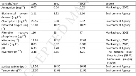
the period of 1992 and to an even lower 47 (μg/L) by 2005 (Mankasingh, 2005). 143
Table 1: Summary of annual average concentrations of environmental variables for the Tamar
144
Estuary (1990-2005). 145
Variable/Year 1990 1992 2005 Source
Ammonium (mg l−1) 0.07 0.04 0.02 Mankasingh, (2005)
Biochemical oxygen
demand (mg l−1
)
2.11 1.52 1.10 Environment Agency
Chlorophyll a (mg l−1
) 29.55 6.98 6.32 Environment Agency
Dissolved oxygen (mg l−1)
10.00 10.76 10.29 Environment Agency
Filterable reactive
phosphorous (μg l−1
)
110 63 47 Mankasingh, (2005)
Nitrate (mg l−1) 11.65 12.10 12.61 Mankasingh, (2005)
Nitrite (mg l−1) 0.03 0.02 0.008 Mankasingh, (2005)
pH 6.33 7.70 7.59 Environment Agency
River flow (m-3/-s) 3.48 8.65 4.01 The National River
Flow Archive (NRFA) Gunnislake gauging station.
Surface salinity (ppt) 17.56 16.30 16.91 Environment Agency
Temperature(°C) 12.10 11.08 11.95 Environment Agency
146
Eden estuary (56022’ N, 2050’ W)
147
In comparison with the Tamar, the Eden Estuary is a small (11km-long) shallow bar built or ‘pocket’ 148
estuary, located between the village of Guardbridge and the town of St Andrews on the East coast of 149
Scotland (Figure 2). Collectively the Eden estuary along with the Firth of Tay Estuary is designated as 150
a Special Area of Conservation (SAC) under the European Union’s Habitats Directive (92/43/EEC) and 151
a Special Protection Area (SPA) under the European Commission Directive on the Conservation of 152
Wild Birds (79/409/EEC). The main channel of the estuary is flanked by relatively wide intertidal 153
areas (8km2) that plays host to large populations of overwintering waterfowl and wading bird 154
species. Historically the intertidal mud and sand flats of the estuary have been sampled intensively 155
[image:5.595.67.530.351.609.2]M
AN
US
CR
IP
T
AC
CE
PT
ED
5
Marine Laboratory (Bennett & McLeod, 1998) providing a robust baseline from which to draw 157
comparisons. 158
159
160
161
162
163
164
165
166
167
168
169
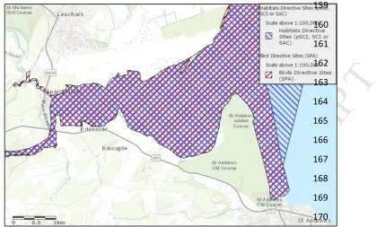
[image:6.595.78.498.108.361.2]170
Figure 2: Map of the Eden Estuary European Marine Site.©Copyright European Environment Agency 171
(EEA). 172
Anthropogenic pressure in the form of increased nutrients from arable and livestock production is 173
one of the most significant pressures influencing the Eden with high levels of nitrogen compounds 174
entering the estuary via the river Eden (Clelland, 1997). Historically this has led to a number of 175
ecological problems such as the closure of mussel beds as unfit for human consumption and 176
widespread fish mortalities (Defew & Paterson, 2009). As a consequence the catchment was 177
designated as a nitrate vulnerable zone in 2003 (SEERAD, 2003). Nutrient inputs are now in decline 178
(Table 2) thanks to increased legislation resulting from the Nitrates Directive (NVZ) and Sensitive 179
Area (UWWTD) designations (Macgregor & Warren, 2015), including an upgrade of the Guardbridge 180
sewage treatment works in 2008 and the closure of the Guardbridge paper mill and adjacent pig 181
farm with their associated effluent. 182
Table 2: Summary of annual average concentrations of environmental variables for the Eden Estuary 183
(1999-2015). 184
Variable /Year 1999 2015 Source
Ammonium (mg l−1) 0.091 0.048 Environment Agency
Chlorophyll a (mg l−1) 10.56 4.28 Environment Agency
Dissolved oxygen (mg l−1) 11.39 10.74 Environment Agency
Filterable reactive phosphorus (mg l−1)
0.23 0.098 Environment Agency
Nitrate (mg l−1) 7.72 5.82 Environment Agency
Nitrite (mg l−1) 0.035 0.015 Environment Agency
pH 7.92 8.11 Environment Agency
River flow (m-3/-s) 2.67 2.13 The National River Flow
Archive (NRFA) Kemback gauging station.
[image:6.595.63.531.568.759.2]M
AN
US
CR
IP
T
AC
CE
PT
ED
6
2.2 Materials & Methods
185
Biomass flow networks (t/km2/yr−1) were constructed for the systems outlined above, using the
186
“Ecopath with Ecosim” software package (v6.5) for the years 1990, 1992 and 2005 (Tamar) and 1999 187
and 2015 (Eden) representing eutrophic and post-eutrophic systems. Ecopath trophic models are 188
mass balance models that create a static snapshot of energy flows and there interactions in an 189
ecosystem represented by trophically linked biomass 'pools' or ecological guilds of species (Pauly et
190
al., 2000). In a model, the energy input and output of all living groups must be balanced. Ecopath 191
parameterizes models based on two master equations one to describe the production term and one 192
for the energy balance of each group (Christensen et al., 2005). The first equation divides the 193
production of each compartment into individual components. This is implemented with the 194
equation: 195
Production = total fishery catch rate + predation mortality + biomass accumulation + net migration + 196
other mortality 197
Or, more formally, 198
B − − − − = 0 Equation 1
199
Where Bi and Bj are the biomasses of prey (i) and predators (j) respectively; P/Bi the
200
production/biomass ratio; EEi the ecotrophic efficiency which describes the proportion of the
201
production that is utilized in the system,; Yithe fisheries catch per unit area and time; Q/Bjthe food
202
consumption per unit biomass of j; DCjithe fraction of prey iin the average diet of predatorj; BAithe
203
biomass accumulation rate for i (the default value of zero was used to indicate no biomass 204
accumulation); and Eiis the net migration of i, calculated as immigration(migration into the area
205
covered by the model) minus emigration(migration out of the area, the default value of zero was 206
used).Within the model, biomass was expressed as tonnes km−2 and production and consumption as 207
tonnes km−2 yr−1. 208
Equation two expresses how the energy balance within each compartment is ensured when 209
consumption by prey biomass = production + respiration + unassimilated food 210
Or, more formally, 211
= x + + Equation 2
212
Where Ri is the respiration rate, and Uithe unassimilated food rate. Respiration is used in Ecopath,
213
only for balancing the flows between groups and refers to the assimilated fraction of matter that is 214
not used in production. Following other estuarine Ecopath models (e.g. Baeta et al., 2011), it is 215
assumed that autotrophs and detritus based organisms have zero respiration with all nutrients that 216
leave the compartment being re-utilized. For each compartment unassimilated food (Ui) consists of
217
food which is egested and flows to the detritus. Following Christensen et al. (2000), our models used 218
a Ui default value of 0.20 for all groups (i.e. 20% of the consumption for all groups).
219
2.2.1 Sampling methods and data collection
M
AN
US
CR
IP
T
AC
CE
PT
ED
7
Chlorophyll a measures provided by the Environment agency (Table 2) for each catchment were 221
transformed into a proxy for phytoplankton biomass using a conversion factor taken from Anderson 222
& Williams (1998). Quantitative biomass data for the main benthic primary producers 223
(microphytobenthos, macroalgae and other macrophytes) at the estuarine scale were made using 224
the Ecopath model based on case study specific estimates of their production, using data from small 225
scale in situ measurements (e.g. Bale et al., 2006) and knowledge of other trophic assemblages.
226
Model biomass estimates were examined and compared with the existing literature to ensure the 227
predations were plausible. For instance, there have been a number of long-term biotope and aerial 228
surveys of saltmarsh and macroalgal extent (Webster et al., 1998; EA., 2000;Widdows et al., 2007; 229
Curtis et al., 2010) on various regions of the Tamar complex. The macroalgal group here is likely to 230
comprise of locally registered species such as Enteromorpha and Ulvae spp. while the ‘other’ 231
macrophyte grouping is likely to comprise a wide variety of seagrass and saltmarsh species such as 232
by not limited to: common saltmarsh-grass (Puccinellia maritime), common cord-grass (Spartina
233
anglica), common eelgrass (Zostera marina), red fescue (Festuca rubra) and sea couch (Elymus
234
pycanthus). 235
To obtain an approximate value for microphytobenthic biomass and production in the Eden system, 236
contact cores were taken across identical transects of each of the three main zones of the estuary in 237
1999 and 2015 by sampling the top 2 cm of the surface sediment (see Ford & Honeywill, 2002 for full 238
protocols). The presence of macroalgae (biomass t km2) was estimated by a survey of macroalgae
239
within 5m radius of each sampling point (Ford & Honeywill, 2002). Macroalgae were mostly 240
identified to be Enteromorpha and Ulvae spp. Estimates of ‘other’ macrophytes in the system were 241
calculated, based on known in situ estimates of saltmarsh extent and production (Fife Council, 2008; 242
Maynard, 2003; 2014; Maynard et al., 2011). Common species represented by this grouping were 243
likely to include common saltmarsh-grass (Puccinellia maritime), sea clubrush (Bolboschoenus
244
maritimus) and the eelgrasses (Zostera augustifolia), (Z. noltii), and (Z. marina). 245
In the Tamar system, invertebrate data from three studies allowed some inter-comparisons to be 246
made at the estuarine scale at similar times of the year, using similar sampling methodologies 247
(Watson et al., 1995; SWW Tamar Estuary sublittoral sediment survey 1992 & Sanders, 2008). In the 248
Eden estuary, extensive surveys of invertebrate data were collected in 2015 through identical 249
surveys to those carried out in 1999 by the BIOPTIS programme (Watson et al., 2018). During this 250
campaign three sampling grids were established across three transitional areas of the estuary 251
(Appendix A). Invertebrate densities for both systems were converted to biomasses using case 252
study-specific relationships (e.g., Dashfield & McNeill, 2014 Tamar & Biles et al., 2002 Eden).
253
Invertebrate species that were not naturally present in one of the years or sites or whose roles in the 254
trophic network were unimportant (biomass < 0.01 t/km2) were not taken into account. 255
Data on demersal fish species and epibenthic crustaceans could not be collected at the estuarine 256
level in each system for practical reasons. However, historical fisheries-independent trawl surveys 257
mainly undertaken by Russel (1973), McHugh et al. (2011) & Dando (2011) reveal a relative temporal 258
consistency in the overall numbers of flatfish and epibenthic crustaceans in the Tamar estuary 259
between historic (1970 & 1980) and contemporary (2009) trawls. Similar observations into the 260
autecology of the brown shrimp (Crangon crangon) by Henderson et al. (1987; 1990) and later by 261
Campos et al. (2008; 2009; 2012) across several British estuaries including the Tamar suggest a 262
consistency in the population structure and phylogeography of this species over our study period. 263
Therefore, given that the spatial structure of the demersal fish and caridean shrimp assemblage has 264
remained relatively constant, similar biomass values for each of these taxa were used over the time 265
periods. Data on fish populations in the Eden were also unattainable from the literature due to a 266
paucity of fish monitoring surveys within the estuarine complex. Demersal fish biomass estimates 267
were therefore estimated by Ecopath, based on P/B. Q/B and EE. Data on epibenthic crustacean 268
numbers, most specifically the brown shrimp (Crangon crangon) were obtained as part of the 269
M
AN
US
CR
IP
T
AC
CE
PT
ED
8
Population numbers for waterbirds in both systems were obtained for the period 1990-2015 from 271
the WeBS (Wetland Birds Survey) database (Frost et al., 2016). Bird counts were based on monthly 272
observations across 15 (Tamar) & 5 sectors (Eden) covering the whole of each respective complex. 273
Twenty-three waterbird species were selected from the Tamar system and Eighteen waterbird 274
species from the Eden system (representing >95% of the total bird numbers in each system, with 275
those excluded largely representing seabird species) from a list of local species known to inhabit and 276
feed on the estuary recurrently, to increase the chance of interoperating temporal changes. Prior to 277
analysis counts were converted to biomasses using species specific body weights outlined by Snow & 278
Perrins (1998). 279
2.2.2 Compartments
280
Some groups of species were grouped into compartments based on similar ecological niches. The 281
benthic-microalgae group here is primarily composed of freshwater and marine diatoms with no 282
single species dominating the community throughout the year. In the case of the Tamar, demersal 283
fish species were amalgamated into one compartment comprising sole (Microstomus kitt), turbot 284
(Phrynorhombus norvegicus), plaice (Pleuronectes platessa) and dab (Limanda limanda). In the 285
Tamar Estuary, the flounder (Platichthys flesus) was considered as a separate compartment being 286
the only ray-finned demersal fish to migrate and colonize the upper reaches of the estuary due to its 287
considerable powers of osmoregulation (Hartley, 1940; 1947). In the Eden Estuary, the demersal fish 288
fish identity was assumed to be a combination of all benthic fish species know to occur within the 289
estuary. In all models, invertebrate species belonging to family Ampharetidae were grouped 290
together, with many of these species sharing a functional role. No data were available for bacteria, 291
therefore the benthic bacterial biomass was considered has being part of the detritus compartment, 292
as recommended by Christensen and Pauly (1992a, b). 293
2.2.3 Ecopath food webs and trophic structure
294
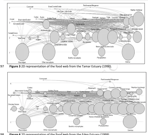
The final versions of the Tamar (Figure 3) and Eden (Figure 4) food webs comprised 43 and 41 taxa 295
M
AN
US
CR
IP
T
AC
CE
PT
ED
9
[image:10.595.41.528.63.508.2]Figure 3 2D representation of the food web from the Tamar Estuary (1990). 297
Figure 4 2D representation of the food web from the Eden Estuary (1999). 298
Whilst phytoplankton and benthic-microalgae are included due to their known importance in 299
structuring benthic ecosystems, other water column elements (zooplankton, planktivorous fish (e.g. 300
shad, sand eel) and their consumers (species in the family Salmonidae) were not included in this 301
model and are considered to follow a separate pelagic trophic pathway (Hall & Raffaelli, 1991).This 302
is due to both planktonic and benthic networks of cycling representing independent domains of 303
control (Baird & Ulanowicz, 1989), with benthic-microalgae constituting a significant proportion of 304
benthic estuarine ecosystem functioning. This model instead centres on a detritus based pathway 305
with particulate organic matter passing through micro-phytobenthos to macro-invertebrates to fish 306
or birds (e.g. Raffaelli, 2011) and a second pathway is also used from macroalgae to macro-307
invertebrates or herbivorous wildfowl (Baird & Milne, 1981). In addition, although the harbour seal 308
(Phoca vitulina) and grey seal (Halichoerus grypus) are known to roam freely through the Eden 309
Estuary (and to a lesser extent the lower Tamar Estuary), they were not included in either modelling 310
framework due to their diets mainly consisting of planktivorous fish (e.g. sandeels, whiting and 311
species of the family Salmonidae) foraged out with the estuarine area in question. For instance 312
Sharples et al., (2009), noted in a study of the diet of harbour seals in the Eden and adjacent St. 313
Andrews Bay to consist of 81 to 94% sandeels in winter and 63% in summer and autumn, with 314
M
AN
US
CR
IP
T
AC
CE
PT
ED
10
2.2.4 Production, consumption and diet composition
316
Production/Biomass ratios required for Ecopath were collected from a number of web-based 317
databases (e.g., Fishbase (Froese & Pauly, 2016) and WeBS database (Frost et al., 2016)). For all 318
vertebrate groups this information was readily available from these databases. For avian species, 319
production was calculated as recruitment (R) of young into the adult population in units per 320
individual (tonnes per year; Stenseth, 2002). For the primary producer and invertebrate groups, 321
Brey’s (2001) Virtual Handbook on Population Dynamics, version 4 (Brey, 2012) was used to 322
calculate the P/B for all species. The weight-to-energy ratios needed in order to apply the empirical 323
method were also provided by Brey (2001). In the case of combined groups the means of each 324
component parameters, were weighted by the relative biomass of the components. For all 325
heterotrophic compartments, Production/ Consumption ratios were entered into the program in 326
order to estimate the Consumption /Biomass ratio’s indirectly. The only exception was in the case of 327
demersal fish species where a holistic predictive model for Consumption/Biomass using asymptotic 328
weight, habitat temperature, a morphological variable and food type as independent variables were 329
calculated using Fishbase 330
Diet matrices were built for each taxa using information from a wide variety of literary sources and 331
summed to unity. Resident invertebrate diet compositions was compiled largely from MBA data 332
holdings including MARLIN and BIOTIC databases while shorebird and flatfish data referenced from 333
the WeBS and Fishbase databases respectively. Complimentary diet information was also gathered 334
from the literature (see Appendix B for all diet references). Initially all species were listed from each 335
taxa along with their percentage contribution to the compartment. Each observed dietary item was 336
then assigned to each individual group of species, with the final percentage of the diet assumed to 337
be proportional to the fraction that its biomass comprised of the total biomass of the functional 338
group. 339
2.2.5 Anthropogenic exports (Yi)
340
A complete mass balanced model needs estimates of the export rates from the system, including the 341
harvesting of economically important species. Commercial flat fishing mortality by means of landings 342
from the Tamar was considered sufficiently small enough to be negligible, based on records of 343
numbers of fish caught of species of 130 mm and upwards (Clark, 2012). Commercial fishing effort 344
on the Eden Estuary was also considered to be minor, with the estuary and surrounding St Andrews 345
Bay protected by a Scottish Inshore Fishing Order (1989) which forbids the use of all mobile fishing 346
gears, including trawling and dredging practices within the area. Similarly the harvesting of 347
commercial invertebrate species such as Cerastoderma edule, Mytilus edulis, Hediste diversicolor,
348
Nephtys hombergii and Crangon crangon for bait fisheries or human consumption was considered
349
insignificant in terms of overall biomass export from the system Tamar (Curtis, 2010) and Eden 350
where bait collection is strictly controlled. 351
352
353
354
355
356
357
M
AN
US
CR
IP
T
AC
CE
PT
ED
11 359
2.2.6 Pre-balancing analysis (PREBAL)
360
To add rigor and validity to the models a set of pre-balance diagnostics (PREBAL) outlined by Link 361
(2010) and recommended by Heymans et al. (2016) were made to assess any issues with the models 362
structure or quality of the primary input data. First the logarithmic ratios of biomass among various 363
taxa groups were plotted (Appendix C) as they have been repeatedly identified as a major indicator 364
of marine ecosystem functioning (Link, 2005; Mokany et al., 2016). Generally biomass 365
decomposition generally followed a sequential decrease moving across trophic levels. While detrital 366
groups where not used it is noted for context that detrital standing stocks were on the same order of 367
magnitude as primary producer biomass, consistent with systems such as estuaries and benthic 368
orientated food webs that are particularly dependent upon detrital energy. In a second step, the 369
vital rates of all taxa, in the form of Production/Biomass ratio and Consumption/Biomass ratio were 370
plotted (Appendix C) for comparison, as these ratios are reflective of an amalgamation of an entire 371
suite of physiological processes. As with the biomass estimates, there was an acceptable decline in 372
vital rates with increasing trophic level. 373
374
2.2.7 Balancing the models
375
Using the ecological and thermodynamic rules for balancing Ecopath models outlined by Darwall et
376
al., (2010)elements of the diet matrix or the values of the three inputted parameters were adjusted
377
iteratively until all logical constraints were met.This was done starting with the lowest quality data 378
first, preserving the most reliable data. In both the Tamar and Eden case studies, the most reliable 379
data were the biomass and production values, and consequently these values were left largely 380
unchanged. Diet matrices were principally unaltered but differed slightly to reflect the known 381
trophic responses of species to different pressures. In all incidences the balancing parameter 382
changes fell within the ranges of uncertainty associated the development of the ‘pedigree’— a 383
routine in Ecopath modelling that quantifies the quality of the input data by assigning confidence 384
intervals based on the origin of the information. The pedigree index P calculated for the Tamar 385
models was 0.481 and 0.593 for the Eden, with the higher latter value reflecting the use of locally 386
collected data and trophic information used to parameterise the models. The various parameters for 387
the balanced Ecopath models of the Tamar and Eden ecosystems are presented in (Appendix D). 388
2.2.8 Summary of system statistics and indices
389
After mass-balancing the models, a number of indices that describe the structure, function and 390
resilience of each system as a whole were calculated using a suite of Ecological Network Analysis 391
(ENA) algorithms incorporated into Ecopath (Christensen et al., 2005). A summary of each index 392
chosen is given in Table 3. 393
394
395
396
397
398
399
M
AN
US
CR
IP
T
AC
CE
PT
ED
12 401
Table 3 Selected Ecological Network Analysis (ENA) indicators
M
AN
US
CR
IP
T
AC
CE
PT
ED
13 403
System Indices Description Units
Sum of all consumption
(Σ C),
Σ C is the sum of all consumption in a system. t km−2 yr−1
Respiratory flows (Σ R) ΣR is the sum of all respiratory flows in a system. t km−2 yr−1
Flows to detritus (Σ FtD) Σ FtD consists of what is egested (the non-assimilated food) and those elements of the groups, which die of old age, diseases, etc.
t km−2 yr−1
Production (Σ P) Σ P is the sum of all production flows in a system. t km−2 yr−1
Total system throughput (TST)
TST represents the entire amount of biomass flow within the system (consumption + export + flows to detritus + respiration) and represents the size of the system (Ulanowicz, 1986). As such, it is an important parameter for comparisons of trophic flow networks
t km−2 yr−1
Total biomass (excluding detritus) (∑B)
Total biomass in the system excluding detritus. t km−2
Total primary
production/total biomass (PP/B),
PP/B, is expected to be a function of the system’s maturity (Odum, 1969). The PP/B ratio can take any positive value and is dimensionless.
Primary
production/respiration (PP/R)
PP/R, is the difference between total primary production and total respiration. It is considered by Odum (1971) to be an important ratio for description of the maturity of an ecosystem.
The PP/R ratio can take any positive value and is dimensionless.
Total throughput cycled (T cycled)
T cycled is the fraction of, an ecosystem's throughput that is recycled. t km−2 yr−1
Finn’s index (CI) CI captures the functions of carbon and nutrient cycling in the system using a proxy of (% of total throughput).
% of total throughput
Predatory cycling index (PI) PI is a slightly modified form of the CI index, computed after cycles involving detritus groups have been removed.
% of throughput w/o detritus
Average path length (APL) APL measures the average number of transfers a unit of medium (e.g. carbon) will experience from its entry into the system until it leaves the system (Baird
et al., 1991).
The APL is a positive
value and is
dimensionless.
The system omnivory index (SOI)
SOI specifies how consumer feeding interactions are distributed across trophic levels. A value close to 0 indicates the consumer is specialised (i.e. it feeds on one trophic level) while a higher value indicates a diet composed of prey across many trophic levels (Christensen et al., 2000).
The SOI is a positive
value and is
dimensionless.
Ascendency (A) A represents both the size and organisation of a system (Ulanowicz, 1986, 1997). Ascendency is a measure of a systems stability and a proxy for a systems resilience.
Flowbits or the product of flow (e.g., t/km -2/year)
Development capacity (C) C represents the upper limit for the size of the Ascendency. Both ascendency and capacity are measures of a systems stability and resilience.
Flowbits or the product of flow
System Overhead (O) O is the difference between capacity and ascendency and is also a measure of system resilience. Higher system overheads indicate that a system has a larger amount of energy in reserve (in flowbits) with which it can use to resist impacts (Ulanowicz, 1986). Overhead is also defined as the pathway redundancy (Ulanowicz, 1997).
M
AN
US
CR
IP
T
AC
CE
PT
ED
14
3 Results and discussion
404
3.1 Statistics of ecological functioning and network structure
405
To quantify the difference within and between the two systems it was necessary to compare the 406
relative magnitude of change in their various system information indices (Table 4). One clear 407
comparison between the networks is that the Tamar is far more active than the Eden, its total 408
system throughput (23464 t km−2 yr−1, 2005, defined as the sum of all flows in the system) is almost 409
25% larger than that of the Eden(17957 t km−2 yr−1, 2015). Some of the higher activity in the Tamar 410
can be attributed to its greater size and freshwater inputs than the Eden, but higher nutrient inputs 411
to the Tamar are also likely to enhance its activity. Because total system throughput scales all 412
information indices, the ascendency and other related variables are uniformly greater for the Tamar. 413
Despite the topological network differences of each system, in both systems, Total biomass 414
(excluding detritus) decreased substantially between the pre and post-management periods. The 415
impact of these changes was reflected by falls in many of the system indices including: consumption, 416
respiratory flows, flows to detritus, and net primary production. There is also evidence that the size 417
(TST) or ‘power’ of each system decreased greatly between the focal periods. These changes were 418
almost certainly attributed to the direct bottom up-effects of nutrient reductions which altered the 419
abundance of benthic primary producers, with cascading consequences on invertebrate and 420
waterbird species at higher trophic levels. These changes were also responsible for changes in 421
secondary production and a number of higher level systems metrics. The effects are believable, not 422
because of a statistically rigorous experimental design, but because the effect sizes are very large, 423
and the altered biodiversity and ecological functioning are clearly different relative to the post 424
management periods. 425
Associated with TST, the network characteristics of the Tamar and Eden ascendency (A), capacity (C) 426
and overhead (O), all decreased considerably by the post-management periods. This is consistent 427
with Ulanowicz’s (1980;86) interpretation that nutrient perturbed systems can be defined by any 428
increase in system ascendency that causes a rise in total system throughput (TST), that more than 429
compensates for any fall in the mutual information content (e.g. A, C or O) of the system. In other 430
words, the greater nutrient inputs tend to simulate a systems growth but despite its augmented 431
activity, its organisation or structure is degraded. 432
Relative ascendency (A/C) was very similar between pre and post-management periods, suggesting 433
that each system was able to accommodate (or resist) the large-scale changes in nutrient loading, 434
primary production, and invertebrate biomass. When only the relative fluxes are concerned, the 435
Tamar Estuary showed a decline of -1.19% in ascendency (A/C) relative to a larger change of -3.66% 436
in internal Ai/Ci by the 2005 period, indicating a higher dependency of this system on connections 437
to adjacent ecological and physical systems (e.g. the Western English Channel). In contrast, internal 438
relative ascendency (Ai/Ci) remained relatively similar between the periods (+0.53%) in the Eden 439
system, indicating that this system has maintained its activity without too much dependence on 440
external system connections. As the degree to which environmental change is likely to influence 441
ecosystem resilience will depend on metacommunity structure and connectance (Dunne et al., 2002; 442
Fung et al., 2015), the (A/C) index could therefore be a suitable indicator to compare ecosystems of 443
different sizes (e.g. Mann et al., 1989, Baird et al., 1991). 444
M
AN
US
CR
IP
T
AC
CE
PT
ED
15
Table 4 Summary of ecological and network statistics/indices for the Tamar and Eden estuarine 446
systems. 447
448
3.2 Cycling structure
449
As making judgment about the trophic status of two entire ecosystems based on a few information 450
indices may seem precarious to some (Ulanowicz, 2004; Fath et al., 2007), comparisons between the 451
Tamar and Eden ecosystems were supported by a broader analysis of the two networks. Support for 452
comparisons were made by considering the trophic structure and cycling pathways contained within 453
the two ecosystems. Because each trophic pathway is a series of interconnected cycles, stressors 454
occurring at any point will disrupt flow to higher levels (Voris et al., 1980; Ulanowicz, 1983). We 455
would expect therefore, that systems with greater resistance to and resilience from nutrient stress 456
to be more complex, in the sense that they contain longer loops of connections that cycle at lower 457
frequencies. Conversely, systems under increased nutrient stress would possess fewer such cycles, 458
due to link disruptions, and each cycle would transfer less medium, particularly to higher trophic 459
levels (Baird & Ulanowicz, 1993). Indeed this is what the comparison shows: the cycles derived from 460
the Tamar and Eden systems were deficient both in number and length under high nutrient levels 461
consistent with hypothesis that systems with longer cycles and low proportions of cycling are 462
indications of less stressed systems. 463
464
Estuary Tamar Eden
Indices 1990 1992 2005 1999 2015 Units
Sum of all consumption (∑ C) 27416 27790 12254 26122 9386 t km−2 yr−1 Sum of all respiratory flows
(∑ R)
16474 16698 7373 15696 5648 t km−2 yr−1 Sum of all flows into detritus
(∑ FtD)
60403 6379 2982 5763 2121 t km−2 yr−1
Sum of all production (∑ P) 11508 10863 7156 8560 3860 t km−2 yr−1
Total system throughput (TST) 54675 55592 23464 50526 17957 t km−2 yr−1
Total biomass (excluding detritus) (∑B)
2680 2617 1703 1926 958 t km−2 yr−1
Total primary production/total biomass (PP/B)
2.320 2.036 2,774 1.74 1.88 -
Total primary production/total respiration (PP/R)
0.367 0.319 0.641 0.21 0.35 -
Ascendency (A) 77715 79561 29844 68252 23523 Flowbits Capacity (Ca) 256513 273649 127706 294697 84797 Flowbits Overhead (O) 178798 194088 97862 226445 108320 Flowbits Relative ascendency (A/C)% 30.02 30.68 31.21 23.16 29.21 % Internal ascendency (IA) 47448 48099 20390 45641 15763 Flowbits Internal capacity (IC) 175004 189876 89455 193430 75478 Flowbits Internal overhead (IO) 127556 141777 69066 147047 59715 Flowbits Internal relative ascendency
(Ai/Ci)%
M
AN
US
CR
IP
T
AC
CE
PT
ED
16
Considering the magnitude of mineral and nutrient cycling within the Tamar system, Finns Index (CI) 465
increased between both periods by ~10 & 30% respectively (Table 5), while the Predatory cycling 466
index (PI) increased initially by 0.18% but then decreased by 0.59%. Together these changes point to 467
a general increase in the detrital cycling process, but a fall in the predatory species contribution to 468
these processes. Networks of cycled flows for the Tamar show that the total number of cycles in the 469
system is sixteen, with these cycles distributed to varying degrees though three cycling nexuses 470
[image:17.595.60.535.181.417.2](cycles having the same smallest transfer is called a nexus (Baird et al.,1991)). 471
Table 5 Cycle distributions of the Tamar and Eden systems 472
Distribution (%) of cycles per nexus Tamar Eden
1990 1992 2005 1999 2015
1 16.67 16.67 16.67 10 10
2 50 50 50 40 40
3 33.33 33.33 33.33 30 30
4 0 0 0 20 20
Number of cycles 16 16 16 10 10
Average path length (API) 2.681 2.716 2.945 2.82 2.90
Throughput cycled (including detritus)t km−2 yr−1 1034 1014 984 1395 754
Throughput cycled (excluding detritus)t km−2 yr−1 290 365 449.34 12.52 33.29
Throughput cycled (by detritus) % 72.76 66.06 93.4 99.02 95.52
Predatory cycling index (PI) % of throughput w/o detritus
0.68 0.86 0.27 0.03 0.24
Finn’s cycling index (CI) % of total throughput 10.90 20.76 40.54 19.08 40.37
473
The API of associated cycles, and throughput of material cycled (including detritus) was fairly 474
consistent across the study period (2.6-2.9 and 1034-984 t km−2 yr−1 respectively), indicating that 475
flows of cycling were consistently occurring over short and fast loops. The percentage of material 476
specifically cycled by the detritus compartment was also proportionately high (>72%), with 477
increasing importance by the 2005 period (>93%). 478
In comparison with the Tamar, the cycling structure of the Eden estuary consisted of a total of ten 479
cycles, distributed to varying degrees though four cycling nexuses (Table 5). The API of associated 480
cycles, was fairly consistent between the study periods (2.8-2.9) specifying that flows of cycling were 481
occurring over short and fast loops. The percentage of material specifically cycled by the detritus 482
compartment was also proportionately very high (>95%), with around about a 4% shift towards non-483
detritus based cycling during the 2015 period. Indices representing the regulating and cycling of 484
nutrients in a system (CI and PI) also increased during the 2015 period, suggesting greater system 485
retentiveness and a greater proportion of material cycled across both higher and lower trophic 486
levels (Odum, 1969). Both estuaries were found to recycle a large proportion of their material 487
though short-fast cycles, with the majority of matter (e.g. carbon) being retained for approximately 488
2-3 cycles. The increasingly high CI index indicates both estuaries have a relatively simple cycling 489
structure with both CI and API of a similar order as other estuaries with a legacy of nutrient 490
contamination e.g. the Ythan Scotland (Baird & Ulanowicz, 199), with a study by Raffaelli (2011) also 491
showing a similar increase in the CI index under a period of nutrient reduction. 492
493
494
M
AN
US
CR
IP
T
AC
CE
PT
ED
17
3.3 A safe operational space
496
In addition to managing stocks and flows, environmental managers often need to know if a 497
particular model projection (or policy option) will push the system being managed into a potentially 498
unsafe state (i.e. whether a system will cross a critical threshold or tipping point). Thus, scientists 499
and managers invested in considering a whole-systems approach may not be interested in the 500
marginal changes of all species (Donohue et al., 2013), but instead whether the system is capable of
501
accommodating potential changes while retaining its capacity to function while remaining within its 502
“safe-operating” space, and hence is resilient (Raffaelli, 2016). While it should be accepted that no 503
single descriptor can fully accommodate the multifaceted nature of ecosystem resilience (Ulanowicz, 504
1992), one possible way to derive system-level measures of resilience, is to adopt a holistic systems 505
approach rather than trying to measure the independent trajectories of several indicators. In 506
particular, Ulanowicz (2011) has argued that the network metric, “ascendency,” has a restricted set 507
of values for real-world ecosystems, where a system lacking ascendency has neither the extent of 508
activity nor the internal organization needed to function sustainably. By contrast, systems that are 509
so tightly constrained and honed to a particular environment appear ‘‘brittle’’ (in the sense of 510
Holling (1986)) are prone to collapse in the face of even minor novel disturbances (Ulanowicz et al.,
511
2009). Systems that endure lie somewhere between these extremes, with such networks falling 512
within a “Window of Vitality” (Ulanowicz, 2005). Further, Zorach & Ulanowicz (2003) have 513
demonstrated that such connections within the “Window of Vitality” can be adequately captured 514
using the structural properties of networks. Thus by plotting such variables, scientists and managers 515
can make a priori predictions about the preferential loss or reduction of stocks (e.g. species, 516
populations, communities), against the effects on ecosystem functioning in relation to a “safe 517
operating space” (Raffaelli, 2015; 2016). Such an approach also allows trade-offs between different 518
network configurations that support different management and policy options be considered (e.g. 519
under the impacts of different nutrient regimes). In this way different modelling scenarios or 520
management choices can be assessed in a cost effective and canonical way, without the need to 521
disturb natural ecosystems (Dunne & Williams, 2009). 522
523
524
525
526
527
528
529
530
531
532
533
534
M
AN
US
CR
IP
T
AC
CE
PT
ED
18 536
Figure 5 The “safe operating zone” (delineated by dotted lines) for the Tamar (Black circles) and 537
Eden (White circles) estuaries defined by ascendency considerations and captured by two simple 538
topological properties of food webs: linkage density and number of trophic levels. 539
Encompassing the changes in ascendency for the Tamar and Eden time periods within Ulanowicz’s 540
“Window of Vitality” (Figure 5), linkage density and number of trophic levels were shown to be very 541
different between the pre- and post-management periods. This would locate the post-management 542
Tamar and Eden periods within the right-hand boundary of the box in Figure 5. In contrast, during 543
the high nutrient periods in both systems graduated towards the top right area of the perimeter 544
space, with the Tamar effectively moving close to leaving the defined “safe operating zone”. Under 545
such circumstances, the results would indicate that the Eden system was able to accommodate 546
historic large scales effects of changes in nutrient loading over the investigated periods, while the 547
Tamar was operating in a relatively unsustainable state in the 1990’s and relative to its less disturbed 548
state in 2005. Implications for the Tamar in its high nutrient state would suggest that some trophic 549
pathways may have narrowed, leaving the system less resilient with insufficient reserves to resist 550
future disturbances (Ulanowicz, 2002). Subsequently both systems have moved closer to the 551
geometric centre of the window (c = 1.25 and n = 3.25) which represents the best possible 552
configuration for system sustainability (Ulanowicz et al., 2009). 553
Overall, the system resilience measures used here suggest that large scale shifts in the nutrient 554
balance of each estuary did not move the systems out of their safe space, which might give grounds 555
for optimism of traditionally high nutrient systems such as estuaries (Leschine et al., 2003; Elliott &
556
Whitfield, 2011). Nonetheless, both versions of the Tamar and Eden networks were close to the 557
“safe” operational boundary during the high nutrient periods and still remain just on the right of the 558
Ulanowicz’s ascendency curve, and at the top left corner of his “Window of Vitality”. The question 559
remains as to whether future stressors acting additively or synergistically with changes in nutrient 560
loading (e.g. increased river flow or water temperatures) could push the systems out of their safe 561
space. By plotting the values of the three variables related to Ulanowicz’s (2005) “Window of 562
Vitality” for many ecosystems under different environmental pressures, it may become possible to 563
identify a region in perimeter space that characterises a generic healthy and robust ecosystem 564
(Raffaelli, 2015). 565
[image:19.595.79.495.73.306.2]M
AN
US
CR
IP
T
AC
CE
PT
ED
19
3.4 Model limitations
567
When interpreting the modelled outputs from this study, several assumptions and limitations of 568
model capability must be considered. Firstly, the development of an Ecopath model strongly 569
depends on the quality of data used to build the model (Christensen & Walters, 2004). In this study, 570
the data for almost all groups (Biomass, P/B, Q/B) were derived from site and time specific raw 571
databases or stock specific assessments providing a solid background for dynamic modelling. 572
However, for groups that play an important role in the Tamar or Eden estuaries food–web but for 573
which no or very little data was available, i.e. certain macrofauna or meiofauna, their omission from 574
the developed ecological networks may have led to an oversimplification in the structure of all food– 575
web components. A specific lack of long term continuous biomass monitoring data in both case 576
study areas, particularly for invertebrates and demersal fish, was also a specific limitation in 577
validating historic trends and improving the validity of future predicted outcomes. Moreover, due to 578
lack of specific knowledge, several functional groups have been aggregated, e.g. demersal fish 579
potentially masking important species interactions (Essington, 2006). Other important factors that 580
this study did not attempt to represent included the variability of future changing climate 581
forcing/environmental or management regimes the adaptive potential of species (e.g. by affecting 582
refuge and breeding space, altering animal behaviour, affecting hydrodynamic transports). While 583
some of these uncertainties could be addressed by further laboratory experiments and in situ
584
monitoring of ecosystem conditions, temporal variations in species-specific habitat factors, e.g. a 585
loss of habitat, cannot be addressed in Ecopath but instead needs a spatial model (e.g. the Ecospace 586
component of Ecopath with Ecosim, Christensen & Walters, 2004). We also acknowledge the need to 587
raise the standards of Ecopath models in a management context (Heymans et al., 2011; 2016), with
588
similar standards needed in exploring ecosystem theory (Pocock et al., 2016). Within the last few 589
years, a growing number of diagnostic checks, including the PREBAL checks used in this paper, have 590
been developed to establish best practices in creating and using such models (Mackinson et al.,
591
2009; Darwall et al., 2010; Link, 2010; Heymans et al., 2016; Scott et al., 2016). These guidelines take
592
into consideration the underlying thermodynamic and ecological rules available to users, 593
recommend approaches to balance an Ecopath model, and how to evaluate uncertainty. In practice 594
if these practices are upheld, it would allow not only more rigorous and consistent models, but 595
would also aid in the acceptance of Ecopath and other mass balance models within science and 596
management. 597
598
4 Conclusions
599
The process of constructing the Ecopath models here provides a valuable end product in itself 600
through explicit synthesis of work from many researchers and has allowed a summarising of our 601
current knowledge of the trophic flows, cycling structure and potential safe operational space of two 602
estuaries with ongoing managing challenges associated with eutrophication. The models also help to 603
highlight potential system specific data gaps (e.g. diet compositions, site-specific P/B, Q/B ratios, fish 604
population numbers), that if collected in the future could be used to enhance and improve the 605
knowledge of each system. The results of the mass balanced models show that the trophic structure, 606
ecological functioning and general resilience of both the Tamer and Eden estuaries were affected 607
similarly following distinct restoration events. This adds further evidence that reducing nutrient 608
inputs to estuarine systems is not only beneficial to the biodiversity elements of a system (Howarth 609
et al., 2011), but also has wider positive implications on a wide range of important system properties 610
which may only be revealed at the system level (Raffaelli, 2006). By understanding the recovery 611
trajectory of individual systems and the metrics that can describe such responses, such information 612
can be of direct relevance to many scientific and regulatory frameworks (Duarte et al., 2015), for
M
AN
US
CR
IP
T
AC
CE
PT
ED
20
example the European Water Framework Directive (WFD) in its pursuit to assess benthic integrity 614
and determining good ecological status (GES). In the systems studied here, the shifts in the vast 615
majority of the structural and functional indicators were generally consistent with recovery 616
trajectories described for other UK and European Ecopath studies on nutrient disturbed systems 617
(Patrício & Marques, 2006;Baeta et al., 2011; Raffaelli, 2011;Selleslagh et al., 2012). This supports
618
the usefulness of ENA type approaches for assessing the recovery patterns of temperate transitional 619
benthic systems. As scientists using the “Ecosystem Approach” are increasingly interested in how 620
different impacts or recovery options will simultaneously change the ecological functioning of a 621
system (Bennett, 2015) we also suggest that the comparison of information indices between 622
networks when complemented by the inherent analysis of cycles can comprise a useful quantitative 623
approach for inter-ecosystem comparisons (Wulff & Ulanowicz, 1989). Moreover, while the use of 624
ENA modelling is extremely useful in establishing possible disturbance effects, one difficulty with the 625
use of ecological models might be translating these results to stakeholders in an effective manner, 626
(Fulton, 2011). As such, transforming process based models into simple graphical descriptions of risk 627
may be useful to illustrate the integrity of the networks to future change. As coastal systems are 628
host to a complex array of interactions between multiple stressors (Jackson et al., 2016), a key next 629
step will be to focus on the underlying processes and mechanisms whereby the stressors affecting 630
these ecosystems interact. 631
632
5 Acknowledgements
633
This work [NERC Grant Ref: NE/K501244/1] was funded with support from the Biodiversity and 634
Ecosystem Service Sustainability (BESS) programme. BESS is a six-year programme (2011-2017) 635
funded by the UK Natural Environment Research Council (NERC) and the Biotechnology and 636
Biological Sciences Research Council (BBSRC) as part of the UK’s Living with Environmental Change 637
(LWEC) programme. This work presents the outcomes of independent research funded by the 638
Natural Environment Research Council through the Biodiversity and Ecosystem Service Sustainability 639
(BESS) programme. The views expressed are those of the author(s) and not necessarily those of the 640
BESS Directorate or NERC. DMP also received funding from the MASTS pooling initiative (The Marine 641
Alliance for Science and Technology for Scotland) and their support is gratefully acknowledged. 642
MASTS is funded by the Scottish Funding Council (grant reference HR09011) and contributing 643
institutions. We are grateful to Dr Sheila Heymans (The Scottish Association for Marine Science, 644
SAMS) and Dr Paul Somerfield (Plymouth Marine Laboratory) for their advice and for providing data 645
for this project. 646
References
647
Allesina, S. & Bondavalli, C., 2004. WAND: an ecological network analysis user-friendly 648
tool. Environmental Modelling & Software, 19(4),337-340. 649
Anderson, T.R. & Williams, P.L.B., 1998. Modelling the seasonal cycle of dissolved organic carbon at 650
station e1in the english channel. Estuarine, Coastal and Shelf Science, 46(1), 93-109. 651
Arreguín-Sánchez, F., & Ruiz-Barreiro, T. M. 2014. Approaching a functional measure of vulnerability 652
in marine ecosystems. Ecological Indicators, (45), 130-138. 653
Baeta, A., Niquil, N., Marques, J. C., & Patrício, J. 2011. Modelling the effects of eutrophication, 654
mitigation measures and an extreme flood event on estuarine benthic food webs. Ecological 655
Modelling, 222(6), 1209-1221. 656
Baird, D., & Milne, H. 1981. Energy flow in the Ythan estuary, Aberdeenshire, Scotland. Estuarine, 657