A. Karabanov, D.C. Rose, W. K¨ockenberger, J.P. Garrahan, and I. Lesanovsky School of Physics and Astronomy, University of Nottingham,
University Park, NG7 2RD, Nottingham, UK and
Centre for the Mathematics and Theoretical Physics of Quantum Non-equilibrium Systems, University of Nottingham, Nottingham NG7 2RD, UK
(Dated: September 8, 2017)
We study an ensemble of strongly coupled electrons under continuous microwave irradiation in-teracting with a dissipative environment, a problem of relevance to the creation of highly polarized non-equilibrium states in nuclear magnetic resonance. We analyze the stationary states of the dy-namics, described within a Lindblad master equation framework, at the mean-field approximation level. This approach allows us to identify steady state phase transitions between phases of high and low polarization controlled by the distribution of disordered electronic interactions. We compare the mean-field predictions to numerically exact simulations of small systems and find good agreement. Our study highlights the possibility of observing collective phenomena, such as metastable states, phase transitions and critical behaviour in appropriately designed paramagnetic systems. These phenomena occur in a low-temperature regime which is not theoretically tractable by conventional methods, e.g., the spin-temperature approach.
Introduction — The control and detection of magne-tization arising from a polarized ensemble of unpaired electron spins forms the basis of electron spin, or param-agnetic, resonance (ESR/EPR); a powerful spectroscopy tool for studying paramagnetic materials placed in a static external magnetic field. The underpinning key principle for this technique is the application of oscillat-ing magnetic fields close to or at the electronic Larmor frequency (usually in the microwave regime) to generate non-equilibrium distributions of populations and coher-ences between quantum states that lead to detectable sig-nals [1–3]. The evolution of systems of isolated or only weakly coupled paramagnetic centres under the effect of these fields is well understood. A more challenging prob-lem is to predict the response of strongly coupled electron ensembles to such perturbations, particularly in samples in the solid state in which anisotropic components of the electronic interactions are not averaged out by thermal motion. Insight into the dynamics of strongly coupled, microwave driven electronic ensembles is also needed in order to improve our understanding of dynamic nuclear polarization (DNP), which is an out-of-equilibrium tech-nique to enhance the sensitivity of nuclear magnetic res-onance (NMR) applications by orders of magnitude (see, e.g., Ref. [4–6]) — in particular, this concerns the cross effect and thermal mixing DNP mechanisms [7–13].
Here we shed light on the non-equilibrium stationary states of a strongly interacting electronic ensemble under continuous microwave driving and subject to dissipation to the environment. We model the dynamics of this sys-tem in terms of a Markovian master equation and use a mean-field approximation to compute the steady state phase diagram. This reveals phase transitions between states of high and low electronic polarisation as well as the emergence of a critical point that displays Ising uni-versality [44]. These features are controlled by the dis-tribution of the disordered electronic spin-spin
interac-tions. The uncovered mean-field transitions imply the emergence of metastable states and accompanying inter-mittent dynamics [17,42, 43], which we confirm numer-ically through simulations of small systems. Our results suggest that under appropriate conditions collective phe-nomena such as metastability, phase transitions and crit-ical behaviour should be observable in driven-dissipative, paramagnetic systems. These predictions complement those of conventional theoretical approaches, based, e.g., on the so-calledspin-temperature which, due to their re-striction to certain parameter regimes, would only pre-dict a homogenous quasi-equilibrium state [10–12, 18– 23].
Model — We model the evolution of the electron sys-tem within the framework of a Markovian Lindblad mas-ter equation. The density matrixρof a system consist-ing ofN microwave-driven electrons evolves according to
˙
ρ = −i[H, ρ] +Dρ. The Hamiltonian H at high static magnetic field, in the rotating frame approximation, is given by
H =X
k
(ω1Skx+ ∆kSkz) + 3
X
k<k0
Dkk0SkzSk0z
−X
k<k0
Dkk0 0Sk·Sk0. (1)
Here ω1 is the strength of the microwave field, ∆k are
the offsets of the electron Larmor frequencies (detun-ings) from the microwave carrier frequency, and Dkk0,
D0
kk0 are coefficients that parameterize the strength of
the anisotropic and isotropic parts of the spin-spin dipo-lar and exchange interactions [3]. Depending on the de-gree of order and symmetries within the sample struc-ture,Dkk0 andD0
kk0 can either be well defined (e.g., for
crystals) or random (e.g., for glasses). In amorphous ma-terials ∆k are also distributed due to the anisotropic
inhomogeneous broadening of the EPR line [3,13,24]. Dissipative processes are modeled by the dissipatorD which describes single-spin relaxation and takes the form
D=X
k
[γ1+L(Sk+) +γ1−L(Sk−) +γ2L(Skz)],
γ1±=
R1
2 (1∓p), γ2= 2R2, p= tanh ~ωS
2kBT
(2)
where L(X)ρ ≡ XρX† −
X†X, ρ /2 is the Lindblad form of a dissipation operator [25]. The dissipation rates depend on the longitudinal (R1) and transversal (R2) relaxation rates of the electron spins as well as the ther-mal polarizationp∈[0,1], which depends on the average electron Larmor frequency ωS and the temperature T.
Note, that throughout the paper many observables will be expressed throughpand thereby acquire their temper-ature dependence. For typical experimental conditions (W-band, ωS ∼100 GHz, sample temperature between T ∼0 K andT ∼100 K)pis in the region of 1−0.01.
Mean-field in the absence of disorder — In order to obtain a basic understanding of the phase structure of the driven electron system, let us first disregard any dispersion in the frequency offsets and interactions, by setting ∆k = ∆ and Dkk0 = D/(N −1). In the
non-disordered case, the last term of Eq. (1) commutes with the rest of the Hamiltonian and does not influence the bulk polarization dynamics. Therefore, we can neglect it, leading to the mean-field Hamiltonian
¯
H =X
k
(ω1Skx+ ∆Skz) +
3D N−1
X
k<k0
SkzSk0z. (3)
We now compute the stationary average bulk polar-ization pz =−2PTr (Skzρss)/N which serves as an
or-der parameter for classifying the steady state ρss and coincides (due to the system homogeneity) with the steady-state polarization of the individual spins. To ob-tain the mean-field equation, we consider the projection
Hk =ω1Skx+ ¯∆kSkz of ¯H onto the subspace of an
ar-bitrary spin k. Here ¯∆k = ∆ + N3D−1Pk06=kSk0z is the
effective energy shift or offset term experienced by the spin that accounts for the frequency offset and interac-tions with other spinsk06=k, which introduces collective effects. This effective (collective) energy shift takes dis-crete values
¯
∆k ∈ δ(q) = ∆ +
3D N−1
q−N−1 2
(4)
where q = 0, ..., N −1 is the number of spins k0 6= k
in the up-state. For each value q, the steady-state po-larization p0z(q) is given by the single-spin formula [see Supplementary Material (SM), A]
p0z(q) =p
1− ηω
2 1 δ2
0+δ2(q)
(5)
whereδ0=pR2
2+ηω12andη=R2/R1is the ratio of the
electron spin relaxation rates. Averaging Eq. (5) over all values ofq(thus taking into account all possible orienta-tions of the surrounding spins) finally yields the equation for the relative steady-state polarization ¯pz=pz/p:
¯
pz=f(∆, D,p¯z)≡ N−1
X
q=0
P(q, pp¯z)p0z(q)/p. (6)
Here P(q, pz) = Nq−1(1−pz) q(1+p
z)N−1−q
2N−1 is the
proba-bility of having q up spins and N −q−1 down spins. Since the right-hand side depends on ¯pz, Eq. (6) should
be regarded as a self-consistency condition. Note also that Eq. (6) depends on ∆,D and temperature (via the thermal polarizationp).
Low and high temperature regime — The relative polarization is bounded (|p¯z| ≤ 1), thus f(¯pz) defines a
continuous map of the unit interval ¯pz ∈ [0,1] to itself.
Therefore, by virtue of the Brouwer fixed point theorem [26], Eq. (6) always has at least one solution. We find that the solution is unique for small values ofpcorresponding to high temperatures and small numbers of spinsN (see SM, B).
For small values of N we can compare the results of the mean-field treatment to the exact solution of the quantum master equation given by the dissipator (2) and Hamiltonian (3). To this end we show in FIG.1(a) the steady-state polarization spectrum, i.e. the depen-dence of the bulk polarization ¯pz on the average
mi-crowave offset ∆, for three typical sets of parameters for
N = 4. Generally a good agreement is obtained. The observed spectra haveN Lorentzian peaks occurring at ∆ = 3D(1/2−q/(N −1)), q = 0,1, . . . , N −1, with a half-width ofδ0. The centre ∆ = 0 of the spectrum
corre-sponds toq∼q0≡(N−1)/2. The mean of the binomial
distributionP(q, pp¯z) where the maximal saturation is
given by ¯q= (N −1)(1−pp¯z)/2. Here ¯q is close to q0
for smallpand tends to shift fromq0 with increasingp.
Hence, the intensities of the peaks are symmetric with respect to the centre of the spectrum at high tempera-tures (p∼0) and undergo a shift from the centre at low temperatures (p∼ 1), with the relation betweenp and the temperature defined through Eq. (2).
Multi-stability and phase transitions — The situ-ation qualitatively changes when entering the regime of low temperatures, i.e. large thermal polarizationp∼1, and high numbers of spins N 1. In this case (see SM, B) Eq. (6) can feature more than one solution. In FIG.1(b)we show the phase diagram given by the num-ber of solutions of Eq. (6) in terms of the scaled offset and interaction parametersa= ∆/ω1
√
η,b= 3D/ω1
√
−20 −10 0 10 20 0.2
0.4 0.6 0.8 1
∆ (MHz)
[image:3.612.68.547.52.149.2]high T medium T low T (b)
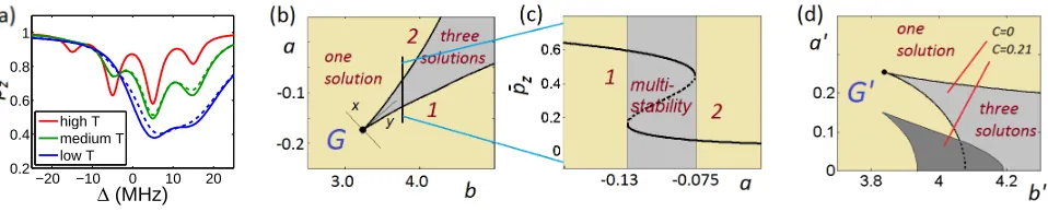
FIG. 1. (a) Steady-state polarization spectra ¯pz(∆) obtained by the mean-field formula (6) (solid lines) and the numerically exact solution (dashed lines) for N = 4, D = 10 MHz, R2 = 106 s−1 and different temperature and microwave parameters:
p= 0.11,ω1 = 75 kHz,R1 = 103 s−1 (red);p= 0.55,ω1 = 12 kHz,R1= 10 s−1 (green);p= 0.99,ω1 = 7 kHz,R1 = 1 s−1 (blue). (b) Phase diagram obtained from Eq. (6) in the (a, b)-plane. The diagram features regions of unique (brown) and multiple (gray) solutions and displays a (cusp) critical pointG at p= 0.99, ω1 =R2 = 105 and R1 = 1 s−1 (forN = 150 electrons). (c) Structure of the solutions along the cutb= 3.75 (D= 6.3 MHz) through the region with multi-stable region featuring three solutions. (d) Phase diagram obtained from Eq. (7) in the (a0, b0)-plane featuring regions of unique and multiple solutions similar to that in panel (b) and a critical point G0 belonging to the same universality class as G (see text for details). The dark gray region illustrates the impact of disorder in the frequency offsets ∆k (inhomogeneous broadening) on the multi-stability region. The strength of the inhomogeneous broadening is parameterized byc(see SM, E for details).
by analyzing the scaling behavior of the polarization ¯pzin
its vicinity. We find two directions that are singled out: one is given by the curve that is tangent to both spinodal lines [see FIG.1(b)], where we find|p¯z−p¯crit| ∼y1/2, with
¯
pcritbeing the value of ¯pzat the critical point. Along the
perpendicular direction we find|p¯z−pcrit¯ | ∼x1/3. These
are the mean-field scalings of the Ising universality class [32, 44]). In other words the direction y can be thought of as being analogous to temperature in the Ising model, where below the critical temperature, i.e. upon cross-ing the critical point, two ferromagnetic states emerge. Within this analogy the perpendicular directionxcan be regarded as magnetic field (see SM, C for further details). Similar phase diagrams have recently been found in other contexts, e.g., for open driven gases of strongly interact-ing Rydberg atoms [27–29,44], laser polarized quantum systems [30], or certain classes of dissipative Ising models [31,42,43].
The behavior of the steady-state polarization ¯pz upon
crossing the multi-stable region is shown in FIG. 1(c). Solutions with small ¯pz ∼0 correspond to non-thermal
quasi-saturated equilibrium states. States with large val-ues ¯pz ∼1 are unsaturated quasi-thermal equilibria. On
crossing the spinodal curve 1 from large negative val-ues of a, the unique stable quasi-thermal steady state continues to exist but two other steady state solutions appear: a stable quasi-saturated and an unstable inter-mediate one as shown in FIG.1(c). Conversely, on cross-ing curve 2 towards large negative values ofa, the unique stable quasi-saturated steady state continues to exist but two other steady states emerge, a stable and an unstable one. Note, that the occurrence of multiple steady state solutions is an artifact of the mean-field approximation which can be interpreted as the emergence of metastable states [42] near first-order phase transitions.
Experimen-tally those may manifest through hysteretic behavior as recently shown in interacting atomic gases [27–29]. We will return to this point further below.
Disordered spin-spin interactions and augmented mean-field— The results so far indicate possible phase transitions in the polarization of the electron system con-trolled by the frequency offset ∆ and the average interac-tion strength D. However, typical sample materials are not single crystals and electrons are arranged randomly, such that the average interaction experienced by an elec-tron is close to zero [13]. In order to take this into account we need an augmented mean-field description which ac-counts for a distribution in the coupling strengths.
Note that when the disorder in either the offsets ∆k or
the interactions Dkk0 is large enough, unitary dynamics
with Hamiltonian (1) is expected to undergo many-body localisation (MBL) [33]. In this case spatial fluctuations in the long-time state can be significant and determined by the disorder and the initial state, which raises the question of the appropriateness of mean-field. However, in the presence of dissipation, cf. Eq. (2), the non-ergodic MBL phase is unstable and the stationary state becomes delocalized [34–36]. This suggests that the mean-field analysis is still appropriate as long as only static (long-time properties) are investigated. The approach to sta-tionarity may nevertheless display transient non-ergodic effect. For other possible connections between MBL and DNP see [23,37].
For the sake of simplicity we assume that the in-teractions D follow a Gaussian distribution, χ(D) = exp(−D2/D2
0)/(
√
πD0), with zero mean and standard
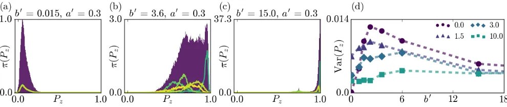
FIG. 2. Numerical simulations and fluctuations. All results in this figure are produced for parametersω1 = 105Hz,R1= 1s−1,
R2 = 105s−1,p= 0.99 andN= 8, and averaged over 10 disorder realizations. (a-c) Discrete approximations of the probability density (dark shaded area) for the observablePzfor three sets of parameters, such that
R
π(Pz)dPz= 1 over the range shown. The light colored curves represent the densities for some individual disorders, divided by the number of disorder realizations considered so that their addition (rather than their average) would equal the full probability density. This is done to better represent the contribution each disorder realization makes to the distribution. Panel (b) shows a strongly broadened distribution signalling enhanced fluctuations. This is consistent with the presence of metastable states that are expected from the mean-field analysis. (d) The variance of the time integrated observablePz for varyingb0, with the fixeda0 value indicated by the legend in the top right.
now. With disorder Eq. (6) generalizes to
¯
pz=
Z +∞
−∞
f0(∆, D,p¯z)χ(D)dD. (7)
To obtain this expression we averaged overχ(D) and ad-ditionally exploited the fact that in the thermodynamic limit (N 1) the function f on the right-hand side of Eq. (6) coincides with the functionf0 =p0z(¯q)/pwhere
¯
q= (N−1)(1−pp¯z)/2 is the mean of the binomial
distri-butionP(q, pp¯z). This givesf0= 1−ηω21/(δ20+δ2) with δ= ∆−3Dpp¯z/2 (see SM, D). The mean-field phase
dia-gram resulting from Eq. (7) is displayed in FIG.1(d)as a function of the dimensionless parametersa0 = ∆0/ω1√η
(∆0 is the average offset, equal to ∆ in the case
con-sidered here) and b0 = 3pD0/2ω1√η. We assume that the strength of the microwave field is large: ω2
1η R22
meaning that the electron system is fully saturated in the absence of spin-spin coupling (in which case the phase transitions observed are most pronounced). The struc-ture is similar to that of FIG.1(b). We observe regions with one and three solutions as well as spinodal lines forming a cusp at a critical pointG0. The scaling prop-erties at this critical point are again those of mean-field Ising universality. Although equal to the non-disordered case the important point is that the underlying mecha-nism is different. In the presence of disorder the phase transition is controlled by the width of the distribution of the disorder strengths (D0∝b0) rather than the average interaction strength, which is in fact zero.
Fluctuations and numerical simulations — The mean-field treatment above is of course not exact. Whether the predicted qualitative phase structure sur-vives away from mean-field depends on the effect of fluc-tuations [31,46]. As shown in [17, 42,43], phase coexis-tence at the mean-field level can be an indication – away from the thermodynamic limit – of the existence of
long-lived metastable (rather than stationary) phases. These competing phases come with an intermittent dynamics of slow switching between them and a significantly longer relaxation time. While the value of the polarization will fluctuate over time within these phases, it will take a distinct average value in each phase. We now show that this is indeed the case by investigating the numerically exact polarization dynamics for a small system, Eqs. (1), (2), by means of quantum jump Monte Carlo simula-tions [45]. In particular we monitor the time dependence of the polarizationpz(t) =−(2/N)PkTr (Skzρ(t)) for a
variety of values ofa0 and b0. For the set of parameters we consider, multiple disorder realizations of the dipolar coupling{Dkk0}, withD0kk0 =Dkk0 are taken. These are
independent and identically distributed, sampled from a Gaussian distribution with variance defined by b0 (see SM, F for details).
Fluctuations due to metastability can be quantified by the probability distribution of the time integrated polarization, Pz = (1/t)R
t 0pz(t
Conclusions — Our results demonstrate that cooper-ative behaviour in strongly interacting ensembles of mi-crowave driven electrons - a situation of relevance to DNP in NMR - can give rise to a non-trivial phase structure in the stationary state of these systems. While the cal-culated phase diagram is mean-field in origin, our sim-ulations show that – even for finite systems – dynamics will be correlated and intermittent, related to the coexis-tence of metastable states. In the future, further insights could be gained by using augmented mean-fields meth-ods for open quantum systems [40]. The experimental demonstration of the predicted phenomena would ideally require a paramagnetic sample with minimal inhomoge-neous broadening, kept at cryogenic temperatures and high magnetic field.
Acknowledgments— The authors thank B. Olmos and J. A. Needham for useful discussions. The research lead-ing to these results has received fundlead-ing from the Eu-ropean Research Council under the EuEu-ropean Union’s Seventh Framework Programme (FP/2007-2013) / ERC Grant Agreement No. 335266 (ESCQUMA) and the EP-SRC Grant No. EP/N03404X/1. We are also grateful for access to the University of Nottingham High Perfor-mance Computing Facility.
SUPPLEMENTARY MATERIAL
This section is the supplementary material (SM) con-taining explanations of the work not fully detailed in the main text.
Steady-state of single-spin microwave-driven dynamics
In the context of our work, the microwave-driven single-spin master equation has the form
˙
ρ=−i[H, ρ] +Dρ
with
H =ω1Sx+δSz,
D=R1
2 [(1−p)L(S+) + (1 +p)L(S−)] + 2R2L(Sz). In terms of the relative polarization components
ρ= 1/2−p(XSx+Y Sy+ZSz),
we come to the Bloch equations (forR2R1)
˙
X =−δY −R2X, Y˙ =δX−ω1Z−R2Y,
˙
Z=ω1Y +R1(1−Z).
0 0.5 1 −0.5
0 0.5 1 1.5
p N=10 20 30 40 50 60
(a)
−200 −10 0 10 20 0.2
0.4 0.6 0.8 1
∆ (MHz)
[image:5.612.321.562.52.141.2]D=0 MHz D=20 D=40 D=60 D=80 D=100 (c)
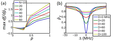
FIG. 3. (a) Dependence of maxdf /dp¯z on the thermal po-larizationpfor different values ofN at ∆ = 10 MHz,D= 20 MHz. (b) High-temperature steady-state polarization spectra for different values ofD, calculated with Eq. (6) forN= 150. In both panels, other parameters are chosen as in the red curve of FIG.1(a) of the main text.
The steady-state solution where the right-hand sides are all zero is unique and calculated as
X = ω1δ
R2 2+δ2
Z, Y =− ω1R2
R2 2+δ2
Z,
Z = 1− ω
2 1η δ2
0+δ2
, δ02=R22+ω12η, η= R2 R1
in full agreement with Eq. (5).
Uniqueness of solution for high temperatures and small
numbers of spins
To understand the structure of the solution space of Eq. (6) as a function of the thermal polarisationpand the number of electrons N, we consider the derivative
df /dp¯z: it is proportional to p, and thus for small
val-ues of p, corresponding to high temperatures, we have
df /dp¯z<1. Under this condition the graph of the
func-tion f(¯pz) can intersect the diagonal g(¯pz) = ¯pz only
once and hence Eq. (6) has only one solution. This high temperatures behaviour is independent of the num-ber of spins N, which is illustrated in FIG. 3(a). Here we plot maxp¯zdf /dp¯z as function ofpfor different values
ofN and fixed other parameters, showing that the max-imum slope for smallpis always negative. The shape of the steady-state polarization spectrum ¯pz(∆) is described
Structure of the phase diagram
Mathematically, the phase diagram of a (smooth) gen-eral two-parametric family of self-consistent relations of the form
u=f(a, b, u), (8)
can be studied from the point of view of the singularities in geometry of the 2-dimensional surface defined by the relation (8) in the 3-space (a, b, u). The relation (8) can be rewritten as
u−f(a, b, u) = ∂F
∂u = 0, F = u2
2 − Z
f(a, b, u)du,
which defines a critical pointuof a (smooth) scalar func-tionF(u) depending on the parametersa, b. This makes a subject of the mathematical theory of singularities com-bined with the geometry of the surface (8) known as the catastrophe theory [41]. The functionF can also be in-terpreted as a “Landau free energy” and the magnitude
uis as an “order parameter”.
Consider the Taylor expansion of Eq. (8) near a given valueu=u∗
u∗+v=f(a, b, u∗+v) =f(a, b, u∗) +∂f
∂u(a, b, u
∗)v+
1 2
∂2f ∂u2(a, b, u
∗)v2+1
6
∂3f ∂u3(a, b, u
∗)v3+. . .≡
c0+c1v+c2v2+c3v3+. . .
If c0 6=u∗ then near the value u=u∗ Eq. (8) does not have solutions. Ifc0=u∗ thenu=u∗ is a solution, and
we have
v=c1v+c2v2+c3v3+. . .
If c1 6= 1 then the solutionu=u∗ is locally unique. If
c1 = 1, c2 6= 0 then u=u∗ is a degeneracy point where two solutions merge,
0 =c2v2+c3v3+. . .
Ifc2= 0,c36= 0 thenu=u∗is a degeneracy point where three solutions merge,
0 =c3v3+. . . ,
etc. Since relation (8) depends on two parameters a, b
and one variableu, in a generic situation no more than three conditions on the coefficients c0, c1, c2 can be si-multaneously satisfied, so not more than three solutions can merge at u= u∗. The latter takes place at the so-called cusp point G of the phase diagram [41] which is defined by the critical valuesa=a∗,b=b∗,u=u∗ with
c0=u∗, c1= 1, c2= 0, c36= 0 (9)
which means
f(a∗, b∗, u∗) =u∗, ∂f ∂u(a
∗, b∗, u∗) = 1,
∂2f ∂u2(a
∗, b∗, u∗) = 0, ∂3f
∂u3(a
∗, b∗, u∗)6= 0.
Consider now the Taylor expansion of Eq. (8) near the cusp point up to terms of the third order, taking into account Eq. (9),
u∗+v=f(a∗+α, b∗+β, u∗+v)∼
u∗+ξ0+ (1 +ξ1)v+ξ2v2+ξ3v3+. . .
which implies
0∼ξ0+ξ1v+ξ2v2+ξ3v3 (10)
with
ξ0= ∂f ∂aα+
∂f ∂bβ+
1 2
∂2f ∂a2α
2+ ∂2f ∂a∂bαβ+
1 2
∂2f ∂b2β
2+
1 6
∂3f ∂a3α
3+1
2
∂3f ∂a2∂bα
2β+1
2
∂3f ∂a∂b2αβ
2+1
6
∂3f ∂b3β
3,
ξ1= ∂
2f
∂u∂aα+ ∂2f ∂u∂bβ+
1 2
∂3f ∂u∂a2α
2+
∂3f ∂u∂a∂bαβ+
1 2
∂3f ∂u∂b2β
2, ξ3= 1
6
∂3f ∂u3,
ξ2= 1 2
∂3f
∂u2∂aα+ ∂3f ∂u2∂bβ
,
where the derivatives off are taken at u=u∗, a=a∗,
b = b∗. The asymptotic cubic equation (10) has three solutions if ¯D <0 and has one solution if ¯D >0, where the discriminant ¯D is given by the expression
¯
D= 1
272ξ6 3
h
3ξ1ξ3−ξ223+
1 4 2ξ
3
2−9ξ1ξ2ξ3+ 27ξ0ξ 2 3
2
= ¯D2+ ¯D3+. . .
where ¯Dnis the term of thenth order inα,β. The lowest
order term is the quadratic term originated fromξ2 0. This
term forms the full square
¯
D2= 1 4ξ2
3
(rα+tβ)2, r= ∂f
Making the rotation on the (α, β)-plane
x=√rα+tβ
r2+t2, y=−
rβ−tα
√
r2+t2
and rewriting the cubic term ¯D3 in the new parameters x, y, we obtain up to the third order
¯
D∼s0x2−s1y3+s2y2x−s3yx2+s4x3
where the coefficientss0−4 are expressed via the
deriva-tives of the functionf(a, b, u) at the cusp point. We have
s0= (r2+t2)/4ξ32>0, so we can write
¯
D∼s0x2
1−s3
s0y+ s4 s0x
−s1y3+s2y2x∼
s0x2−s1y3+s2y2x.
In other words, the critical curve ¯D= 0 is asymptotically represented by the equation
s0x2−s1y3+s2y2x= 0.
The last term can be removed by a shift transformation
x→x+O(y2) and neglecting a term∼y4, so this curve
is asymptotically written as
s0x2−s1y3= 0 : y=
s
0 s1
1/3
x2/3.
This equation defines a cusp curve on the (x, y)-plane with two branches tangent to they-axis at the cusp point
G, see FIG.4(a)where the local geometry of the singular surface (11) is shown. In the rotated local coordinates, the cubic equation (10) representing the relation (8) takes the form
¯
v3−y¯¯v−x¯= 0, x¯= 2s10/2x, y¯= 3s11/3y. (11)
Inside the cusp region s0x2−s1y3 < 0, Eq. (11) has
three solutions, outside the cusp regions0x2−s1y3 >0
only one solution exists. On crossing the cusp point G
along the y-axis, the unique solution ¯v = 0 forks into three solutions ¯v = 0 and ¯v = ±y¯1/2. On crossing G
along the x-axis, the unique solution has a singularity ¯
v =x1/3. The described asymptotics are universal, i.e.,
valid for any two-parametric relation (8) as soon as it has a critical point where relations (9) hold [41].
The critical point Gof the phase diagram of Eq. (6) satisfying Eq. (9) was found numerically to be
a∗∼ −0.18, b∗∼3.23, pcrit¯ ∼0.27
with the characteristic directions in the (a, b)-plane
x∼0.99(a−a∗)−0.14(b−b∗),
[image:7.612.321.552.54.322.2]y∼0.99(b−b∗) + 0.14(a−a∗).
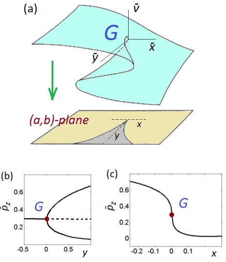
FIG. 4. (a) Universal two-parametric phase diagram consid-ered from the point of view of the mathematical catastrophe theory. (b) Structure of the solutions ¯pz of Eq. (6) on cross-ing the critical pointGalong the tangent direction y. Two stable solutions separated by∼y1/2 are forked from the in-termediate solution that loses its stability. (c) The shape of the solution ¯pz on crossing the critical point along the per-pendicular directionx, with a singularity∼x1/3.
In FIG. 4(b), the structure of the solution ¯pz is shown
on crossing the critical pointGalong the tangent direc-tion y, in FIG. 4(c) — the same on crossing along the perpendicular directionx.
The critical point G0 of the phase diagram of Eq. (7) corresponds to
a0∗∼0.26, b0∗∼3.83, p¯0crit∼0.20
with the characteristic directions (not plotted)
x0∼0.97(a0−a∗0) + 0.25(b0−b0∗),
y0 ∼0.97(b0−b0∗)−0.25(a0−a0∗).
Link to the classical meanfield theory of the Ising model
As shown in the main text, the projection of the av-eraged Hamiltonian of Eq. (3) to the subspace of a ran-domly chosen spinkis written as
where
¯
∆k = ∆ +
3D N−1
X
k06=k
Sk0z.
The classical meanfield theory consists in replacing each operatorSk0zby its bulk steady-state observable (see, for
example, [42–44])
−pz 2 =
1
N
X
k
Tr (Skzρ).
This leads to the single-spin Hamiltonian
˜
H =ω1Sx+ ¯∆Sz, ∆ = ∆¯ −3Dpp¯z/2.
Applying Eq. (5) justified in Appendix , we obtain for the relative steady-state polarization
¯
pz=f0(¯pz), f0= 1− ω21η δ2
0+ ¯∆2
. (12)
Up to differences in notations, this is the classical self-consistent relation for the steady-state of the Ising model driven by a transversal field [42–44].
The same result is obtained if we replace in Eq. (6) the summation over all q by a single mean value of the binomial distributionP(q, pp¯z)
¯
q= (N−1)1−pp¯z
2 .
Indeed,
δ(¯q) = ∆ + 3D
N−1
¯
q−N−1 2
= ¯∆, p
0
z(¯q) p =f0.
To justify the proceeding from the whole set q = 0, 1, . . . , N−1 to the mean ¯q, rescale the integer variable
qby a new variableby the rule
q = q
N−1 (13)
whereq = 0,1/(N−1), . . . ,1 defines a uniform
subdi-vision of the unit interval. The probability density of the variable q is the same binomial distribution P(q, pp¯z)
and the detuningδbecomes a function of ,
δ(q) = ∆ + 3D
q−
1 2
≡δ0(q).
Due to rescaling (13), the mean and the variance of the distributionq are the mean and the variance of the
dis-tributionP divided by (N−1) and (N−1)2respectively,
so we obtain
¯
=
N−1
X
q=0
qP(q, pp¯z) =
(N−1)(1−pp¯z)
2(N−1) =
1−pp¯z
2 ,
σ2 =
N−1
X
q=0
(q−¯)2P(q, pp¯z) =
(N−1)(1−p2p¯2 z)
4(N−1)2 =
1−p2p¯2 z
4(N−1).
In the limit N 1, the variance σ2
becomes zero, so
the distribution q is reduced to a single mean value ¯
taken with the probablity 1. The summation overq can be replaced by an integration over the unit interval with the probablity density represented by the Dirac delta-function ˜δ(−¯),
f(¯pz) = N−1
X
q=0
P(q, pp¯z)p0z(q)/p=
Z 1
0
˜
δ(−¯)
1− ω
2 1 δ2
0+δ
02
()
d=
p0z(¯q)/p=f0.
This justifies the classical meanfield theory (12) as a thermodynamic N 1 limit of the meanfield theory developed in the main text.
Effect of inhomogeneous broadening
To estimate the effect of inhomogeneous broadening, we considered a system represented by two Gaussian spin packets of the same zero mean and standard deviation
D0separated by a difference 2∆0between the detunings. Here the Gaussian densityχ(D) in Eq. (7) remains un-changed while the functionf0(D,p¯z) is modified as
f00(D,p¯z) =
1
2(f+(D,p¯z) +f−(D,p¯z)),
f±(D,p¯z) = 1− ηω2
1 δ2
0+δ±2
, δ±= ∆±∆0− 3Dpp¯z
2 .
The effect of ∆0 6= 0 can be estimated varying the di-mensionless parameterc= ∆
0
ω1√η. For c6= 0, the phase
Quantum Jump Monte Carlo simulations
The simulations for FIG. 2 of the main text were done using the Quantum Jump Monte Carlo algorithm [45] to calculate the stochastic evolution (trajectory) of the pure state of the system over time. While all trajectories are initialized in the same state, the all up configuration, data from a trajectory is only considered after sufficient time has elapsed that there is no memory of the initial state (we can be certain such a time scale exists for this finite system due to the results of [46]), i.e. after the relaxation time. The remainder of the trajectory is then cut up in to time periods T of O(10−2s), chosen such that short time fluctations are averaged out so that only long time fluctuations influence the variance of the time integrated observable (similar to the approach used in Sec. III E of [42]).
Different disorder realizations are handled as follows: we begin by taking a set of random numbers from a Gaus-sian distribution of unit variance, defining the realization. For a given value of b0 we then rescale all of these num-bers by the associated value of the standard deviation
D0. As it can be shown that the probability density
satisfiesp1(x)dx=pD0(D0x)d(D0x) where the subscript
represents the variance of the Gaussian, this rescaling provides us with an equivalent set of numbers that were effectively drawn from a distribution with standard de-viationD0.
[1] E. Zavoisky, J. Phys.9, 211 (1945). [2] G. Lancaster, J. Mater. Sci.2, 489 (1967).
[3] A. Schweiger and G. Jeschke, Principles of Pulse Elec-tron Paramagnetic Resonance (Oxford University Press, 2001).
[4] R. G. Griffin, T. F. Prisner, and C. P. Slichter (ed.), Phys. Chem. Chem. Phys.12, 5725 (2010).
[5] A. V. Atsarkin and W. K¨ockenberger (ed.), Appl. Magn. Reson.43, 1 (2012).
[6] W. T. Wenckebach, Essentials of Dynamic Nuclear Polarisation (The Netherlands Sprindrift Publications, 2016).
[7] A. Kessenikh, V. Luschikov, and A. Manenkov, Phys. Solid State8, 835 (1963).
[8] C. F. Hwang and D. A. Hill, Phys. Rev. Lett.19, 1011 (1967).
[9] K. N. Hu, H. H. Yu, T. M. Swager, and R. G. Griffin, J. Am. Phys. Soc.126, 10844 (2004).
[10] M. Borghini, Phys. Rev. Lett.20, 419 (1968).
[11] V. A. Atsarkin and M. I. Rodak, Phys.-Usp. 15, 251 (1972).
[12] A. Abragam and M. Goldman,Nuclear Magnetism: Or-der and DisorOr-der (Oxford Clarendon Press, 1982). [13] A. Karabanov, G. Kwiatkowski, C. U. Perotto,
D. Wi´sniewski, J. McMaster, I. Lesanovsky, and
W. K¨ockenberger, Phys. Chem. Chem. Phys.18, 30093 (2016).
[44] M. Marcuzzi, E. Levi, S. Diehl, J. P. Garrahan, and I. Lesanovsky, Phys. Rev. Lett.113, 210401 (2014). [43] C. Ates, B. Olmos, J. P. Garrahan, and I. Lesanovsky,
Phys. Rev. A85, 043620 (2012).
[42] D. C. Rose, K. Macieszczak, I. Lesanovsky, and J. P. Garrahan, Phys. Rev. E94, 052132 (2016).
[17] M. Foss-Feig, P. Niroula, J. T. Young, M. Hafezi, A. V. Gorshkov, R. M. Wilson, and M. F. Maghrebi, arXiv:1611.02284 (2016).
[18] B. N. Provotorov, J. Exp. Theor. Phys.14, 1126 (1962). [19] V. A. Atsarkin, Phys.-Usp.21, 725 (1978).
[20] S. Jannin, A. Comment, and J. van der Klink, Appl. Magn. Reson.43, 59 (2012).
[21] Y. Hovav, A. Feintuch, and S. Vega, Phys. Chem. Chem. Phys.15, 188 (2013).
[22] S. C. Serra, A. Rosso, and F. Tedoldi, Phys. Chem. Chem. Phys.14, 13299 (2012).
[23] A. D. Luca and A. Rosso, Phys. Rev. Lett.115, 080401 (2015).
[24] C. P. Poole and H. A. Farach, Bull. Magn. Reson.1, 162 (1979).
[25] A. Karabanov, D. Wi´sniewski, I. Lesanovsky, and W. K¨ockenberger, Phys. Rev. Lett.115, 020404 (2015). [26] L. E. J. Brouwer, Mathematische Annalen71, 97 (1911). [27] C. Carr, R. Ritter, C. G. Wade, C. S. Adams, and K. J.
Weatherill, Phys. Rev. Lett.111, 113901 (2013). [28] N. R. de Melo, C. G. Wade, N. ˇSibali´c, J. M. Kondo,
C. S. Adams, and K. J. Weatherill, Phys. Rev. A93, 063863 (2016).
[29] D. Weller, A. Urvoy, A. Rico, R. L¨ow, and H. K¨ubler, Phys. Rev. A94, 063820 (2016).
[30] A. A. Zvyagin, Phys. Rev. B93, 184407 (2016). [31] H. Weimer, Phys. Rev. Lett.114, 040402 (2015). [32] N. Goldenfeld, Lectures on Phase Transitions and the
Renormalisation Group (Addison-Wesley, 1992). [33] R. Nandkishore and D. A. Huse, Ann. Rev. Cond. Mat.
Phys.6, 15 (2015).
[34] E. Levi, M. Heyl, I. Lesanovsky, and J. Garrahan, Phys. Rev. Lett.116, 237203 (2016).
[35] M. V. Medvedyeva, T. Prosen, and M. ˇZnidariˇc, Phys. Rev. B93, 094205 (2016).
[36] M. H. Fischer, M. Maksymenko, and E. Altman, Phys. Rev. Lett.116, 160401 (2016).
[37] A. De Luca, I. Rodr´ıguez-Arias, M. M¨uller, and A. Rosso,Phys. Rev. B94, 014203 (2016).
[46] S. G. Schirmer and X. Wang, Phys. Rev. A81, 062306 (2010).
[45] A. J. Daley, Adv. Phys63, 77 (2014).
[40] J. Jin, A. Biella, O. Viyuela, L. Mazza, J. Keeling, R. Fazio, and D. Rossini,Phys. Rev. X6, 031011 (2016). [41] V. I. Arnold,Catastrophe theory(Springer Verlag, 1984). [42] D. C. Rose, K. Macieszczak, I. Lesanovsky, and J. P.
Garrahan, Phys. Rev. E94, 052132 (2016).
[43] C. Ates, B. Olmos, J. P. Garrahan, and I. Lesanovsky, Phys. Rev. A85, 043620 (2012).
[44] M. Marcuzzi, E. Levi, S. Diehl, J. P. Garrahan, and I. Lesanovsky, Phys. Rev. Lett.113, 210401 (2014). [45] A. J. Daley, Adv. Phys63, 77 (2014).