Frequency domain subpixel registration using HOG phase correlation

(1)

Elsevier Editorial System(tm) for Computer Vision and Image Understanding

Manuscript Draft

Manuscript Number: CVIU-16-93R1

Title: Frequency domain subpixel registration using HOG Phase Correlation

Article Type: Research paper

Keywords: Phase Correlation; registration in frequency domain; subpixel; Fourier; Histogram of Oriented Gradients.

Corresponding Author: Dr. Vasileios Argyriou, PhD

Corresponding Author's Institution: Kingston University First Author: Vasileios Argyriou, PhD

Order of Authors: Vasileios Argyriou, PhD; Georgios Tzimiropoulos Abstract: We present a novel frequency-domain image registration technique, which employs histograms of oriented gradients providing subpixel estimates. Our method involves image filtering using dense Histogram of Oriented Gradients (HOG), which provides an advanced

representation of the images coping with real-world registration problems such as non-overlapping regions and small deformations. The proposed representation retains the orientation information and the corresponding weights in a multi-dimensional representation. Furthermore, due to the overlapping local contrast normalization characteristic of HOG, the proposed Histogram of Oriented Gradients - Phase Correlation (HOG-PC) method improves significantly the estimated motion parameters in small size blocks. Experiments using sequences with and without ground truth including both global and local/multiple motions demonstrate that the proposed method outperforms the state-of-the-art in frequency-domain motion estimation, in the shape of phase correlation, in terms of

(2)

Dear Review Coordinator,

We would like to submit the attached manuscript, “Frequency domain subpixel registration using HOG

Phase Correlation,” for consideration for possible publication in Elsevier Computer Vision and Image

Understanding journal.

This paper has not been published or accepted for publication from another journal or conference.

The major contributions of this paper include a novel high-performance version of the phase

correlation algorithm based on histogram of oriented gradients (HOG-PC).

Sincerely,

Vasileios Argyriou

Kingston University London

Faculty of Science, Engineering and Computing.

Penrhyn Road

Kingston upon Thames

Surrey KT1 2EE, UK

Email:

[email protected]

Phone: +44 (0) 208 417 2591

(3)

Frequency domain subpixel registration using

HOG Phase Correlation

June 14, 2016

1 General Comments

We would like first to thank the reviewers for their valuable comments and suggestions.

2 Reviewer #1

In this paper, combination of histograms of oriented gradients (HOG) and phase

correlation was used for image registration, which is a reasonable extension of phase

correlation approach for more robustness. Although slightly improved results are

reported, the paper needs address the following issues to improve its presentation.

1) The motivation: as the improvement in comparison to other approaches is

less significant, the author need further justify the motivation of the combination;

The main motivation of our work is to propose a dense HOG-based PC method for sub-pixel

translation estimation that is also invariant to small deformations, and performs well when the

assumption for translation invariance breaks. To the best of our knowledge this is one of the

most important problems in block-based motion estimation, as the problem of noise has been

addressed by many authors in the past. The robustness and accuracy of the proposed scheme

is particularly evident when small blocks (8

×

8) are used. Please notice that in this case (see

tables 1, 4, 7 and Figs 5-10), the proposed HOG phase correlation significantly outperforms

other methods.

More details were added in line 45,

The main point of this work is to propose...

2) Need compare the complexity with other relevant algorithms, especially those

from Ren, GC, NGC and Xiaohua.

Comments on the complexity of the relevant algorithms were added and a new table with

times was included (line 306, table 14).

Overall the complexity of the proposed HOG-PC is higher compared to the other approaches

due to the computational power required for the pre-processing stage and the estimation of the

dense HOG transform. In the current architecture we did not considered any parallel

implemen-tation but if a GPU HOG [1] was used it could be no actual difference among them. [1] Victor

Prisacariu and Ian Reid, “FastHOG - a real-time GPU implementation of HOG”, Department

of Engineering Science, Oxford University”, 2310/09”, 2009

3) Show results from Ren in Figs 11, 13 and Fig 14. You can test on cases with

more noise for better comparisons

(4)

All the above figures were updated including more noise (pages 21, 26 and 27). In the case

of real videos the proposed method outperforms the other methods. Regarding the MRI images

since the image/block size is significantly higher most of the approaches are very close in terms

of accuracy with Ren’s method to outperform especially in very large levels of noise.

4) Show results under different noise rather than Gaussian

Experiments were performed using different levels of motion blur noise. From the obtained

results it can be observed that the proposed HOG-PC method outperforms the others especially

in very small block sizes.

The updates are in lines 250 and 301,

Furthermore, experiments with motion blur present

were performed...

and tables 4-9.

Furthermore, experiments were performed with 8 different levels of motion blur. In each

case...

and table 13.

5) Any way to extend the proposed approach to deal with other motions such

as rotation and zooming?

Thank you for the suggestion, this is something that we have also thought about, however it

is not clear how to apply the principles of scale and rotation estimation in the frequency domain

for multi-channel representations like the dense HOG (for up to 2-channel representation one

can use a complex number representation). This is an interesting extension and we hope to

pursue it in the future.

6) If the estimated motion is block by block, how do you distinguish from

back-ground motion and foreback-ground motion? Also will you do block by block motion

compensation?

We did not consider to distinguish foreground background motion in this work and more

details were added explaining that the estimated motion is block based and that the motion

compensation was block by block too.

7) Check the format and English usage.

(5)

3 Reviewer #2

This paper presented a new motion estimation method by combining the power of

HOG representation and phase correlation. Generally this paper is well written

and easy to follow. I have one concern regarding the computational time, which

is an important factor in video processing. However, I didn’t see the results on

computation cost.

As it was mentioned above comments on the complexity of the relevant algorithms were

added and a new table with times was included (line 306, table 14).

Overall the complexity of the proposed HOG-PC is higher compared to the other approaches

due to the computational power required for the pre-processing stage and the estimation of the

dense HOG transform. In the current architecture we did not considered any parallel

implemen-tation but if a GPU HOG [1] was used it could be no actual difference among them. [1] Victor

Prisacariu and Ian Reid, “FastHOG - a real-time GPU implementation of HOG”, Department

of Engineering Science, Oxford University”, 2310/09”, 2009

Please give more detail information about the medical images used in the last

experiment. For example, what is the image resolution, are they 3D images or the

video clip? In medical imaging, it is very difficult to get the ground truth. Please

explain how do you obtain the ground truth in sub-voxel accuracy.

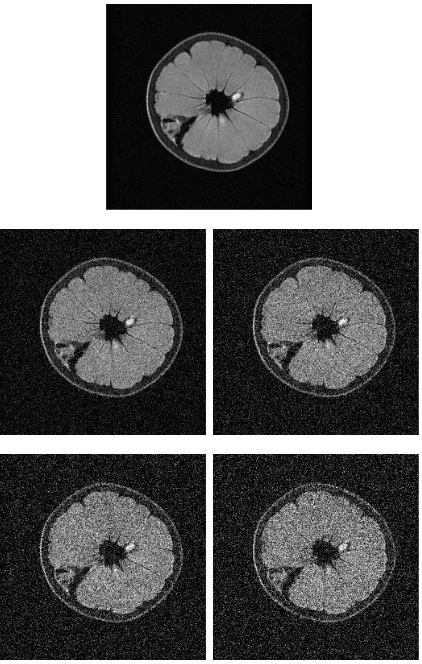
More details on the MRI images were added in line 218.

The images show real MRI data from a grapefruit that was acquired using a production quality

Fast Spin Echo (FSE) sequence on a GE (Faireld, CT, USA) Signa Lx 1.5 Tesla MRI scanner.

The

256 ×

256 pixel images cover a 16

cm

2

_{FOV corresponding to a 0.0625mm square per pixel.}

Five images were acquired with the fruit at dierent positions in the FOV, by manually moving

the scanner table.

Also, Gaussian noise is not common in real clinical applications. On the contrary,

the noise is highly related with machine (scanner). Actually motion blur is more

common than noise. It would be great if the authors can show the motion estimation

accuracy in that scenario.

As it was mentioned above experiments were performed using noise generated by blur filter.

From the obtained results it can be observed that the proposed HOG-PC method outperforms

the others especially in very small block sizes.

The updates are in lines 250 and 301,

Furthermore, experiments with motion blur present

were performed...

and tables 4-9.

Furthermore, experiments were performed with 8 different levels of motion blur. In each

(6)

Highlights

A dense HOG Phase Correlation method

Invariant to small deformations

Performs well when the assumption for translation invariance breaks

The robustness and accuracy is particularly evident when small blocks

(7)

Frequency domain subpixel registration using

HOG Phase Correlation

Vasileios Argyriou and Georgios Tzimiropoulos

Kingston University and University of Nottingham

Abstract

We present a novel frequency-domain image registration technique, which

em-ploys histograms of oriented gradients providing subpixel estimates. Our method

involves image filtering using dense Histogram of Oriented Gradients (HOG),

which provides an advanced representation of the images coping with real-world

registration problems such as non-overlapping regions and small deformations.

The proposed representation retains the orientation information and the

cor-responding weights in a multi-dimensional representation. Furthermore, due

to the overlapping local contrast normalization characteristic of HOG, the

pro-posed Histogram of Oriented Gradients - Phase Correlation (HOG-PC) method

improves significantly the estimated motion parameters in small size blocks.

Experiments using sequences with and without ground truth including both

global and local/multiple motions demonstrate that the proposed method

out-performs the state-of-the-art in frequency-domain motion estimation, in the

shape of phase correlation, in terms of subpixel accuracy and motion

compen-sation prediction for a range of test material, block sizes and motion scenarios.

Keywords: Phase Correlation, registration in frequency domain, subpixel,

Fourier, Histogram of Oriented Gradients.

1. Introduction 1

A critical component of various high-level computer vision and video pro-2

cessing systems is motion estimation and registration. To perform image reg-3

istration, we usually assume that the input images are related by a parametric 4

(8)

geometrical transformation. Then, in order to obtain the unknown motion pa-5

rameters, an optimisation approach is applied on a matching criterion. Pure 6

translation is assumed in this work, which is fundamental in a number of appli-7

cations such as standards conversion, noise reduction, image super-resolution, 8

medical image registration, restoration, and compression. In such systems, mo-9

tion compensated prediction is widely used for filtering and redundancy re-10

duction purposes. International standards for video communications such as 11

MPEGx and H.26x employ motion compensation prediction, which is based on 12

regular block-based partitions of incoming frames. 13

Recently there has been a lot of interest in motion estimation techniques op-14

erating in the frequency domain. Perhaps the best-known method in this class is 15

phase correlation [1, 2], which has become one of the motion estimation methods 16

of choice for a wide range of professional studio and broadcasting applications 17

[3]. Phase Correlation (PC) and other frequency domain approaches (that are 18

based on the shift property of the Fourier Transform (FT)) offer speed through 19

the use of FFT routines and enjoy a high degree of accuracy featuring several 20

significant properties: immunity to uniform variations of illumination, insen-21

sitivity to changes in spectral energy and excellent peak localization accuracy. 22

Furthermore, it provides sub-pixel accuracy that has a significant impact on mo-23

tion compensated error performance and image registration for super-resolution 24

and other applications, as theoretical and experimental analyses have suggested 25

[4]. Sub-pixel accuracy mainly can be achieved through the use of bilinear in-26

terpolation, which is also applicable to frequency domain motion estimation 27

methods. 28

One of the main issues of frequency domain registration methods is that in 29

order to obtain reliable motion estimates large blocks of image data are required. 30

Although this requirement is not an issue when there is a single motion, it causes 31

problems when multiple motions are present and affects the accuracy and the 32

overall motion compensated error (especially at the motion borders). On the 33

other hand, reducing the block size increases the sensitivity to noise and reduces 34

(9)

selecting useful and reliable features is essential. In computer vision and image 36

processing, histogram of oriented gradients (HOG) [5] is a feature descriptor 37

that is invariant to geometric and photometric transformations used mainly for 38

object recognition. Histogram of oriented gradients describe local shapes within 39

an image by the distribution of intensity gradients. The image is divided into 40

cells, and for the pixels within each cell, a histogram of gradient directions is 41

calculated. The local histograms can be normalized by calculating a measure 42

of the intensity across a larger block over a set of neighbouring cells providing 43

invariance to changes in illumination and shadowing. 44

The main point of this work is to propose a dense HOG-based PC method 45

that is invariant to small deformations, and performs well when the assumption 46

for translation invariance breaks. To the best of our knowledge this is one of 47

the most important problems in block-based motion estimation, as the problem 48

of noise has been addressed by many authors in the past. Additionally, the 49

limitations of frequency based methods when small blocks are used is key part 50

of the motivation of the combination, since HOG transform provides an extra 51

advantage in very small block sizes. In more details, in this paper we introduce 52

a novel high-performance version of the phase correlation algorithm based on 53

histogram of oriented gradients (HOG-PC). The key advances introduced by 54

this paper are the use of a dense histogram of oriented gradients to represent 55

the images. Note that the proposed dense representation is quite different from 56

the traditional representation of a block (or patch) based on HOG. The lat-57

ter achieves invariance to small translational displacements and hence does not 58

appear to be suitable for motion estimation. In contrast, we propose to use 59

a very dense representation by calculating a descriptor per pixel. This allows 60

us to interpret the obtain representation as a multi-channel block representa-61

tion. Then, motion estimation is performed by correlating the multi-channel 62

representations from two blocks. Our main contribution lies in showing that 63

this representation not only can recover translational motion very accurately 64

but is also better able to cope with real-world registration problems such as 65

(10)

due to the overlapping local contrast normalization characteristic of HOG, the 67

proposed HOG-PC method improves significantly the estimated motion param-68

eters in smaller size blocks. Finally, subpixel accuracy is obtained through 69

the use of simple interpolation schemes [6, 7]. Experiments with ground truth 70

data, noisy MR images, and real video sequences have shown that our scheme 71

performs significantly better than recently proposed subpixel extensions to the 72

phase correlation method. 73

This paper is organised as follows. In Section 2, we review the state-of-the-74

art in sub-pixel motion estimation using phase correlation. In Section 3, we 75

discuss the principles of the proposed HOG-PC and the key features of this 76

method are analysed. In Section 4 we present experimental results while in 77

Section 5 we draw conclusions arising from this paper. 78

2. Related work 79

In this section, a brief review of current state-of-the-art Fourier-based meth-80

ods for image registration is presented [8]. In many practical encoder implemen-81

tations, sub-pixel motion estimation is achieved by straightforward extensions 82

to the baseline integer-pixel block-matching algorithm mainly through the use of 83

bilinear interpolation. Interpolation in the data domain is also applicable to fre-84

quency domain motion estimation methods such as phase correlation. Moreover 85

such an approach cannot provide estimates of true floating-point accuracy, only 86

approximations to the nearest negative power of two. To circumvent the above 87

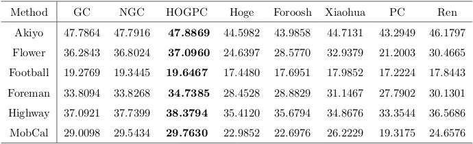
difficulties associated with interpolation, alternative approaches have been de-88

veloped. 89

Recently, several subpixel extensions have been proposed [9, 10, 11, 12, 13, 90

14]. In [15], Hoge proposes to perform the unwrapping after applying a rank-1 91

approximation to the phase difference matrix. In more detail, Hoge presents 92

a so-called Subspace Identification Extension method, which is based on the 93

observation that a ‘noise-free’ phase correlation matrix (i.e. a matrix computed 94

(11)

[image:11.612.166.446.123.415.2]

Figure 1: An example of the dense HOG features represented with orientation histograms

(top) and a obtained correlation surface (bottom).

For a “noisy phase correlation matrix (i.e. a matrix computed from consecu-96

tive frames of a moving sequence), the sub-pixel motion estimation problem can 97

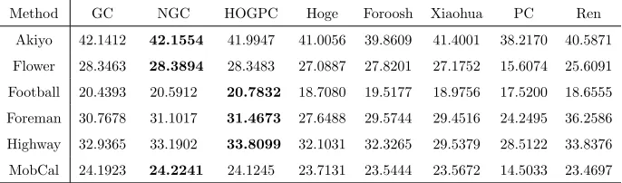
be recast as finding the rank one approximation to that matrix. This can be 98

achieved by using Singular Value Decomposition (SVD) followed by the identifi-99

cation of the left and right singular vectors. These vectors allow the construction 100

of a set of normal equations, which can be solved to yield the required estimate. 101

The work in [16] is a noise-robust extension to [15], where noise is assumed to be 102

AWGN. The authors in [17] derive the exact parametric model of the phase dif-103

ference matrix and solve an optimization problem for fitting the analytic model 104

(12)

[image:12.612.185.428.121.369.2]

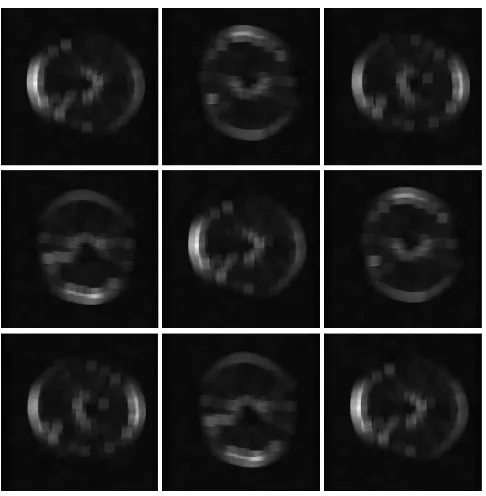
Figure 2: The firstθ= 9 channels of the dense HOG that were used in the proposed HOG-PC.

To estimate the subpixel shifts, Stone et al. [18] fit the phase values to a 2-D 106

linear function using linear regression, after masking out frequency components 107

corrupted by aliasing. The method inevitably requires 2-D phase unwrapping 108

which is a difficult ill-posed problem, while the parameters controlling masking 109

are arbitrarily chosen and require fine tuning. Thus, after obtaining an integer-110

precision alignment of the input images their method takes steps towards alias 111

cancellation by eliminating certain spectral components of each of the two input 112

images. Elimination is based on two criteria: (i) radial distance of a spectral 113

component from the component located at the origin and (ii) magnitude of 114

a spectral component in relation to a threshold. The latter is dynamically 115

determined as follows. Spectral components are sorted by magnitude and are 116

progressively eliminated starting with the lowest. The authors claim that there 117

exists a range in which the accuracy of the computed motion estimate becomes 118

stable and independent of the degree of progressive elimination. This stability 119

(13)

operation on the frequencies that have survived the above two criteria yields 121

the required motion estimates. An extension to the method for the additional 122

estimation of planar rotation has been proposed in [19]. 123

Foroosh et al. [20] showed that the phase correlation function is the Dirich-124

let kernel and provided analytic results for the estimation of the subpixel shifts 125

using thesincapproximation. According to [20], images mutually shifted by a 126

sub-pixel amount can be assumed as having been obtained by an integer pixel 127

displacement on a higher resolution grid followed by subsampling. This assump-128

tion allows the analytic computation of the normalised cross-power spectrum as 129

a polyphase decomposition of a filtered unit impulse. The authors demonstrate 130

that the signal power of the resulting phase correlation surface is not concen-131

trated in a single peak but is distributed to several coherent peaks adjacent to 132

each other. The authors further show that this amounts to a Dirichlet kernel, 133

which can be closely approximated by a sinc function. This approximation 134

allows for the development of a closed-form solution for the sub-pixel shift esti-135

mate. 136

Finally, a fast method for subpixel estimation based on FFTs has been pro-137

posed in [21]. Notice that the above methods either assume aliasing-free images 138

[20, 22, 21, 17], or cope with aliasing by frequency masking [18, 16, 15, 19], 139

which requires fine tuning. 140

3. HOG-PC for Subpixel Registration 141

LetIi(x),x= [x, y]T ∈ R2_,_i_{= 1}_,_{2 be two image functions, related by an}

142

unknown translationt= [tx, ty]T ∈ R2

143

I2(x) =I1(x−t) (1)

To estimate the translational displacement, we use phase based correlation 144

schemes. Each image Ii(x) can be considered as a continuous periodic im-145

age function with periodTx=Ty = 1, [23]. The Fourier series coefficients ofI

146

are given by 147

FI(k) =

Z

Ω

(14)

[image:14.612.201.412.123.455.2]

Figure 3: An example of the MRI data without and with noise of different levels

(0.01,0.02,0.03,0.04).

where Ω ={x:−1/2≤x≤1/2}, k= [k, l]T ∈Z2 andω0= 2π. If we sample

148

Iat a rateN with a 2-D Dirac comb functionD(x) =P

sδ(x−s/N), we obtain

149

a set ofN×N discrete image valuesI1(m) =I(m/N), m= [m, n]T ∈ R2and

150

−N/2≤m< N/2, [23]. UsingD, we can write the DFT of I1 as

(15)

[image:15.612.200.412.121.398.2]

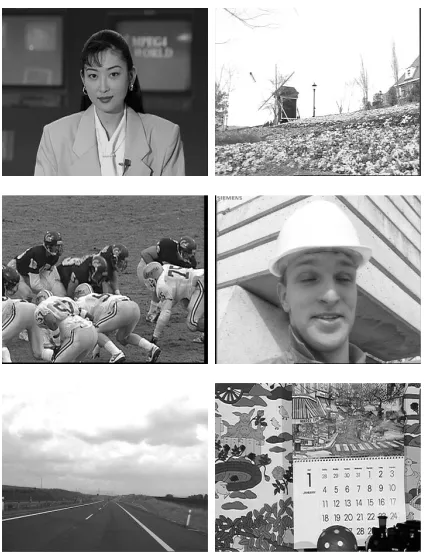
Figure 4: A frame of each video sequence that was used in our evaluation process.

ˆ

I1(k) = X

m

I1(m)e−j(2π/N)k

T_m

=

Z

Ω

D(x)I(x)e−j(2π/N)kTxdx

=FI(k)?X s

e−j(2π/N)kTs/N

=N2X s

FI(k−sN) (3)

where−N/2≤k< N/2 and? denotes convolution. 152

Moving to the shifted version of the image [23], given by the equation (1) 153

witht= [tx, ty]T_,_{_t_:₋₁_{< N}_t_<₁_}_{. Sampling with}_D _{in a similar fashion we}

154

getI2 and its DFT is given based on the Fourier shift property by

155

ˆ

I2(k) =N2 X

s

(16)

[image:16.612.135.479.151.255.2]

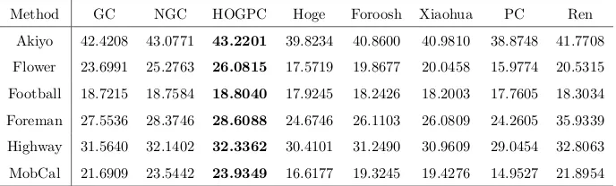
Table 1: Average PSNR (dB) values for all the video sequences and block size 8×8.

Method GC NGC HOGPC Hoge Foroosh Xiaohua PC Ren

Akiyo 42.4208 43.0771 43.2201 39.8234 40.8600 40.9810 38.8748 41.7708

Flower 23.6991 25.2763 26.0815 17.5719 19.8677 20.0458 15.9774 20.5315

Football 18.7215 18.7584 18.8040 17.9245 18.2426 18.2003 17.7605 18.3034

Foreman 27.5536 28.3746 28.6088 24.6746 26.1103 26.0809 24.2605 35.9339

Highway 31.5640 32.1402 32.3362 30.4101 31.2490 30.9609 29.0454 32.8063

MobCal 21.6909 23.5442 23.9349 16.6177 19.3245 19.4276 14.9527 21.8954

Akiyo 43.1677 43.2094 43.1455 43.1980 41.4381 41.8490 41.2989 41.0237

Flower 28.3028 28.5663 28.7076 23.8995 25.9038 25.3230 15.7029 24.4162

Football 19.6813 19.7728 20.0338 18.1636 18.6105 18.4471 17.6603 18.5527

Foreman 29.5387 29.7872 30.2192 25.9039 27.3208 28.0282 24.2521 36.3688

Highway 32.5355 32.8818 33.6166 31.3321 31.7945 30.7668 28.5041 32.8148

MobCal 24.5285 24.8592 24.9101 21.7679 23.0760 23.6421 14.6892 22.7079

Assuming no aliasing and combining equations (3) and (4) we have 156

ˆ

I2(k) = ˆI1(k)e−j(2π/N)k

T₍_N_t)

(5)

Note that the well-known shift property of the DFT refers to integer shifts 157

and does not assume aliasing-free signals. Hereafter, we assume that our sam-158

pling device eliminates aliasing. Traditionally to estimate the translational dis-159

placement, we use phase correlation (PC), which is perhaps the most widely 160

used correlation-based method in image registration. It looks for the maxi-161

mum of the phase difference function which is defined as the inverse FT of the 162

normalized cross-power spectrum [1] 163

PC(u)_,F−1 (

ˆ

I2(k) ˆI1∗(k)

|Iˆ2(k)||Iˆ1∗(k)| )

=F−1{ejkTt}=δ(u−t) (6)

where∗denotes complex conjugate and F−1_{the inverse Fourier transform.}

[image:16.612.135.479.294.395.2]

(17)

[image:17.612.135.478.151.252.2]

Akiyo 42.1412 42.1554 41.9947 41.0056 39.8609 41.4001 38.2170 40.5871

Flower 28.3463 28.3894 28.3483 27.0887 27.8201 27.1752 15.6074 25.6091

Football 20.4393 20.5912 20.7832 18.7080 19.5177 18.9756 17.5200 18.6555

Foreman 30.7678 31.1017 31.4673 27.6488 29.5744 29.4516 24.2495 36.2586

Highway 32.9365 33.1902 33.8099 32.1031 32.3265 29.5379 28.5122 33.8376

[image:17.612.134.478.305.410.2]

MobCal 24.1923 24.2241 24.1245 23.7131 23.5444 23.5672 14.5033 23.4697

Table 4: Average PSNR (dB) values for all the video sequences (50 first frames) and block

size 8×8 with 0.75 variance motion blur.

Akiyo 46.9358 47.9122 48.1894 43.8985 44.0877 43.5653 43.4136 46.3062

Flower 28.4947 30.4891 31.5629 22.6101 24.8113 22.4272 21.7711 26.0737

Football 18.2997 18.2785 18.3126 17.3936 17.6461 17.3321 17.3271 17.8680

Foreman 31.4301 32.5690 33.3006 28.3002 29.1089 28.1744 27.9264 30.5642

Highway 36.2005 36.8582 37.1551 34.6884 35.0371 34.3573 33.5344 36.0504

MobCal 25.3502 27.3564 27.6531 20.4433 22.0091 20.0361 19.5922 23.6230

3.1. Proposed methodology for HOG-PC

165

In this section, we introduce the proposed phase correlation algorithm based 166

on histogram of oriented gradients (HOG-PC). Note that the proposed dense 167

representation is quite different from the traditional representation of a block 168

(or patch) based on HOG. The latter achieves invariance to small translational 169

displacements and hence does not appear to be suitable for motion estimation. 170

In contrast, we propose to use a very dense representation by calculating a de-171

scriptor per pixel. This allows us to interpret the obtain representation as a 172

multi-channel block representation. Then, motion estimation is performed by 173

correlating the multi-channel representations from two blocks. Our main contri-174

bution lies in showing that this representation not only can recover translational 175

motion very accurately but is also better able to cope with real-world registra-176

(18)

[image:18.612.133.478.164.269.2]

Akiyo 47.7864 47.7916 47.8869 44.5982 43.9858 44.7131 43.2949 46.1797

Flower 36.2843 36.8024 37.0960 24.6397 28.5770 32.9379 21.2003 30.4665

Football 19.2769 19.3445 19.6467 17.4480 17.6951 17.9852 17.2224 17.8443

Foreman 33.8094 33.8268 34.7385 28.4528 28.8829 31.1467 27.7902 30.1301

Highway 37.0921 37.7399 38.3794 35.4120 35.6794 34.8676 33.3544 36.5686

[image:18.612.133.480.321.423.2]

MobCal 29.0098 29.5434 29.7630 22.9852 22.6976 26.2229 19.3175 24.6576

Akiyo 47.2598 47.0844 46.9395 42.8979 43.2420 45.2531 42.8459 45.1704

Flower 37.7471 37.7145 37.5289 34.4633 31.8037 35.6403 21.0538 33.7585

Football 20.0454 20.2501 20.4676 17.9476 17.4846 18.2341 17.0028 17.5864

Foreman 34.4031 34.5012 35.1448 29.4785 28.9129 32.9204 27.6481 29.9641

Highway 38.3238 38.8231 39.3635 36.4025 36.3173 34.2663 33.3791 36.9849

MobCal 29.3901 29.4741 29.3422 27.5164 23.2643 27.5576 18.9994 25.1790

noise. Furthermore, due to the overlapping local contrast normalization char-178

acteristic of HOG, the proposed HOG-PC method improves significantly the 179

estimated motion parameters in smaller size blocks. Finally, subpixel accuracy 180

is obtained through the use of simple interpolation schemes [6, 7]. 181

We first describe the traditional HOG descriptor. HOG uses the normalized 182

combination of gradient vectors from a given number of pixels to build up a 183

histogram of binned angles that relate to the feature. The process begins by 184

breaking the image up into set features spacesf comprised of a number of cells 185

c, which in turn is made up of pixels. For each pixel within a cell the filter mask 186

[−1,0,1] is applied to its neighbouring pixels giving us the gradient vector~g. 187

(19)

[image:19.612.133.478.164.267.2]

Akiyo 50.2757 51.0925 51.3390 47.4929 47.0069 47.3463 47.2890 49.0431

Flower 31.4674 32.8165 33.3934 27.2786 27.6245 27.2046 26.9964 29.2145

Football 19.4725 19.3277 19.3736 18.5606 18.6270 18.5354 18.5142 18.8796

Foreman 32.3824 33.2128 33.7498 29.9563 29.9954 29.8935 29.6478 31.4852

Highway 38.8627 39.1613 39.4571 37.5952 37.3573 37.5161 36.8784 38.2206

MobCal 28.1125 29.4835 29.6976 24.4869 24.6221 24.3584 24.1381 26.2775

Akiyo 51.4247 51.3765 51.6485 47.3513 46.8294 50.0535 47.1346 48.8104

Flower 38.2331 39.0902 39.7536 27.5034 27.9538 35.9841 27.0223 29.7296

Football 20.2406 20.3819 20.6140 18.4652 18.5598 19.0224 18.4073 18.7527

Foreman 34.5928 34.2964 35.3176 29.8665 29.7574 33.3645 29.6204 30.9343

Highway 40.1471 40.3989 41.0301 37.7915 37.6942 38.7673 36.9909 38.5279

MobCal 31.6078 32.2799 32.4236 24.8317 24.6213 29.8854 24.1093 26.2672

expressed using angleθ.

θ= tan−1(gy, gx) (7)

Additionally a weight w is defined for each pixel, which is used to scale its 188

contribution to its cell’s histogram. This is given by the mean value of the pixels 189

within a given 2D kernel indicating the density over this area. By applying this 190

weight, the proposed approach provides accurate estimates also in the presence 191

of noise. 192

Once these values are established the pixels within each cell are binned into 193

a histogramH according to theirθ angle. The value added to a bin is given as 194

the weighted magnitude of the vectorwk~gk. Finally all cell histograms within 195

a multi-dimensional featureHj are normalised using theL2 norm.

[image:19.612.135.479.320.424.2]

(20)

[image:20.612.133.478.164.268.2]

Akiyo 51.2539 50.7153 50.6264 40.8783 46.4685 49.6346 46.6632 47.7458

Flower 43.1483 42.6464 42.5386 30.6144 28.6057 41.1037 27.2853 30.8018

Football 21.1975 21.3593 21.7731 18.5759 18.3757 18.6508 18.2522 18.5016

Foreman 35.4305 35.2909 36.2796 29.6047 29.6118 33.8368 29.4914 30.6552

Highway 41.0594 41.7453 42.0343 37.8387 38.3018 39.9322 37.2725 39.0443

MobCal 33.2915 33.2234 33.2526 26.9309 24.4869 30.5041 24.1541 26.2379

Hj→

Hj p

k~gk2 2+e2

(8)

The obtained features are then vectorised as aθ−dimensional descriptor

~

d={H1, ..., Hθ} (9)

Having defined HOG for a single cell, we now turn to the proposed dense 197

HOG representation. For Ii, i = 1,2, we extract d from (9) at each pixel 198

locationIi(m): 199

Hi(m) ={Hi,1(m), Hi,2(m), ..., Hi,θ(m)} (10)

The resulting histograms can be re-arranged as a multi-channel feature repre-200

sentation (see figures 1 and 2). 201

To estimate the subpixel shifttfrom (1) using HOG-PC, we simply compute 202

the correlation between the two multi-channel representation: 203

HOGP C(m) =

θ X

j=1

H1,j(m)? H2,j(−m) (11)

and findt= arg maxmHOGP C(m). We can estimate sub-pixel accuracy

reg-204

istrationt0= (x0, y0) by fitting a 1Dkernel to the vicinity of the maximum on

205

the correlation surface. A parametric kernel is used, which can adapt its shape 206

(21)

Frame No

0 50 100 150

PSNR (dB) 30 32 34 36 38 40 42 44 46 48

50 Akiyo (8x8)

GC NGC Hoge Foroosh PC HOGPC Xiaohua Ren Frame No

0 50 100 150 200 250 300

PSNR (dB) 32 34 36 38 40 42 44 46 48

50 Akiyo (16x16)

GC NGC Hoge Foroosh PC Xiaohua Ren HOGPC Frame No

0 50 100 150 200 250 300

PSNR (dB) 25 30 35 40 45

50 Akiyo (32x32)

[image:21.612.162.449.125.357.2]

GC NGC Hoge Foroosh PC Xiaohua Ren HOGPC

Figure 5: The PSNR values for the Akiyo sequence versus the frame number for all the block

sizes.

subpixel shifts. Based on the work in [23] a reasonable choice for our kernel is 208

given by 209

K1D(x;{x0,p}) =p1{1−(p2(x−x0))2}

1 √

2πp3 e

−(x−x0 )2 2p2

3 (12)

which is a simple modification of the mexican hat wavelet [24]. To estimatey0,

we set up a similar problem with the kernel defined as

K1D(y;{y0,q}) =q1{1−(q2(y−y0))2}

1 √

2πq3 e

−(y−y0 )2

2q₃2 ₍₁₃₎

Our algorithm estimates the kernel parameters{x0,p= [p1, p2, p3]T}and{y0,q=

210

[q1, q2, q3]T}in a least-squares sense.

211

4. Results 212

To evaluate and illustrate the efficiency of the proposed scheme a compar-213

(22)

Frame No

0 50 100 150 200 250

PSNR (dB) 14 16 18 20 22 24 26 28

30 Flower (8x8)

0 50 100 150 200 250

PSNR (dB) 14 16 18 20 22 24 26 28 30 32

34 Flower (16x16)

0 50 100 150 200 250

PSNR (dB) 14 16 18 20 22 24 26 28 30

32 Flower (32x32)

[image:22.612.161.449.124.359.2]

Figure 6: The PSNR values for the Flower sequence versus the frame number for all the block

sizes.

niques. Both data with ground truth and video sequences have been used for 215

evaluating the performance. A set of MRI images are employed which have 216

undergone sub-pixel displacement and it is available by the authors in [15] (see 217

figure 3). The images show real MRI data from a grapefruit that was acquired 218

using a production quality Fast Spin Echo (FSE) sequence on a GE (Faireld, 219

CT, USA) Signa Lx 1.5 Tesla MRI scanner. The 256×256 pixel images cover a 220

16cm2 _{FOV corresponding to a 0.0625mm square per pixel. Five images were}

221

acquired with the fruit at dierent positions in the FOV, by manually moving the 222

scanner table. Regarding the real videos the well-known sequences of ‘Akiyo’, 223

‘Flower’, ‘Football’, ‘Foreman’, ‘Highway’ and ‘MobCal’ were used including 224

150−300 frames each (see figure 4). 225

4.1. Video sequences without ground truth

226

Regarding the real video sequences without ground truth, in order to eval-227

(23)

Frame No

0 50 100 150 200 250 300

PSNR (dB) 14 16 18 20 22 24 26 28 30

32 Football (8x8)

0 50 100 150 200 250 300

PSNR (dB) 14 16 18 20 22 24 26 28 30 32

34 Football (16x16)

0 50 100 150 200 250 300

PSNR (dB) 14 16 18 20 22 24 26 28 30 32

34 Football (32x32)

[image:23.612.161.449.124.358.2]

Figure 7: The PSNR values for the Football sequence versus the frame number for all the

block sizes.

motion compensated sequence is considered. It is defined as the closeness be-229

tween the motion compensated frames and the original ones, and the peak signal 230

to noise ratio (PSNR) is used in this work defined by 231

P SN R= 10 log

₂₅₅2 M SEI

(14)

whereM SEI is the mean square error of the original and motion compensated 232

frames. 233

The performance of the proposed HOGP C scheme is compared with more 234

than five popular P C based methods [15, 20, 22, 6, 17, 7, 23, 9]. Foroosh’s 235

method [20] estimates the subpixel shifts by fitting asincfunction to the avail-236

able correlation samples. Hoge’s and Xiaohua’s [15, 14] methods are based on 237

frequency masking, phase unwrapping and linear regression, while Ren’s [22] 238

approach applies a linear weighting of the height of the main peak on the one 239

(24)

Frame No

0 50 100 150 200 250 300

PSNR (dB) 15 20 25 30 35

40 Foreman (8x8)

0 50 100 150 200 250 300

PSNR (dB) 15 20 25 30 35

40 Foreman (16x16)

0 50 100 150 200 250 300

PSNR (dB) 15 20 25 30 35

40 Foreman (32x32)

[image:24.612.161.449.124.358.2]

Figure 8: The PSNR values for the Foreman sequence versus the frame number for all the

block sizes.

In the second part of our evaluation process, experiments were performed 241

using read video sequences and applying block based motion estimation. The 242

selected block sizes were 32×32, 16×16 and 8×8 pixels and the motion 243

compensated prediction error was estimated for each block size over all the 244

sequences. The average PSNR values are shown in Tables 1,2 and 3 and it can 245

be observed that the proposed approach results the highest values indicating 246

better visual quality. In figures 5, 6, 7, 8, 9, and 10 the PSNR values over time 247

for the video sequences are shown with the proposed scheme to be the most 248

accurate and consistent in comparison with the other state-of-the-art methods. 249

Furthermore, experiments with motion blur present were performed indicating 250

the accuracy of the proposed method especially in the case of small block sizes 251

(e.g. 8×8). The average PSNR values are shown in Tables 4,5 and 6 for motion 252

blur variance equal to 0.75 and in Tables 7,8 and 9 for motion blur variance 253

(25)

Frame No

0 50 100 150 200 250 300

PSNR (dB) 22 24 26 28 30 32 34

36 Highway (8x8)

0 50 100 150 200 250 300

PSNR (dB) 22 24 26 28 30 32 34

36 Highway (16x16)

0 50 100 150 200 250 300

PSNR (dB) 22 24 26 28 30 32 34

36 Highway (32x32)

[image:25.612.160.449.124.357.2]

Figure 9: The PSNR values for the Highway sequence versus the frame number for all the

block sizes.

Finally, in figure 11 we can see the gain of theHOGP C method as a ratio 255

over the other approaches moving from larger to smaller block sizes. As it 256

was expected the ratio increases due to the characteristics of our scheme and 257

HOG. So, since HOG is utilising neighboring information (i.e. surrounding 258

cells) even for small blocksHOGP Cscheme contains more information allowing 259

more accurate estimates especially if larger motions are present. Furthermore, 260

observing the results in Tables 1,2 and 3 focusing on the proposed method and 261

especially for the Akiyo sequence that is characterised of small motion vectors 262

in average, it shows that HOGPC provides the best results for the case of 8×8 263

pixels. Also, it outperforms other methods used over larger blocks such as 16×16 264

pixels, indicating the accuracy of the proposed HOGPC method that exploits 265

(26)

Frame No

0 50 100 150

PSNR (dB) 12 14 16 18 20 22 24 26

28 Mobile Calendar 15fps (8x8)

0 50 100 150

PSNR (dB) 12 14 16 18 20 22 24 26

0 50 100 150

PSNR (dB) 12 14 16 18 20 22 24

[image:26.612.161.449.124.358.2]

Figure 10: The PSNR values for the MobCal sequence versus the frame number for all the

block sizes.

4.2. Real data with ground truth

267

In the case that ground truth is available, the mean square error (MSE) 268

between the estimated subpixel motion vectors and the ground truth is used 269

as a performance measure. Considering two vectorsuand v representing the 270

original (ground truth) and the estimated one, respectively, then 271

M SEM V = 1

n X

i=x,y

(ui−vi)2 (15)

Consequently, a good quality estimate is expected to minimize MSE, which 272

provides the accuracy of the estimates. 273

In more details, a set of five 256×256 pixel real MR images [15] was used 274

and a sample of them is shown in figure 3. The 5 images yield a total of 10 275

possible pairwise registrations and the ground truth of the subpixel translations 276

(27)

Block Size

8x8 16x16 32x32

PSNR Ratio of HOGPC over the other methods

1 1.02 1.04 1.06 1.08 1.1 1.12 1.14 1.16

1.18 Averaged over all Video Sequences

[image:27.612.188.416.128.317.2]

GC NGC Hoge Foroosh HOGPC Xiaohua Ren

Figure 11: The PSNR ratio of the proposed HOGPC scheme over all the other methods for

the different block sizes.

The estimated shifts and the corresponding measurements of their average 278

MSE are shown in Tables 4-12. Observing the results, the proposed method 279

provides the most accurate overall estimates with the lowest mean square error. 280

Furthermore, since ground truth measurements can be significantly biased [15]; 281

the performance of each method was assessed by computing the peak signal-to-282

noise ratio (PSNR) of the motion compensated prediction error. Figure 12 shows 283

the obtained results for each method and all the image pairs. The proposed 284

scheme achieves marginally the best registration accuracy in comparison with 285

N GC [23], while the difference with the other methods is higher. 286

Additionally, the five MR images were used to evaluate the performance of 287

each method in the presence of additive white Gaussian noise. In this case we 288

assume that the correct shift is given by the corresponding noise-free estimate 289

for each method and image pair. In figure 13 the mean value of the registration 290

error for noise variance in the range [0.005,0.045] is illustrated for each method. 291

Observing the results it can be seen that the proposed method is one of the most 292

(28)

[image:28.612.151.464.162.420.2]

Table 10: Average MSE with the corresponding PSNR values, and the estimated motion

vectors for the 10 image pairs of the MRI data (Part 1).

Image pairs [1,2] [1,3] [1,4] [1,5]

GT (-2.40,4.00) (-4.80,8.00) (-7.20,4.32) (-7.20,12.00)

Hoge (-2.03,4.01) (-4.13,8.01) (-6.81,4.17) (-6.82,12.02)

Foroosh (-2.22,4.23) (-4.36,8.24) (-6.59,4.41) (-6.59,12.26)

Balci (-2.11,4.10) (-3.90,8.05) (-6.22,4.34) (-6.39,12.15)

Gaussian (-2.07,4.02) (-4.33,8.01) (-6.57,4.37) (-6.57,12.06)

Quadratic (-2.03,4.01) (-4.18,8.00) (-6.73,4.25) (-6.74,12.03)

Sinc (-2.00,4.00) (-4.12,8.00) (-6.72,4.12) (-6.73,12.00)

ESinc (-2.00,4.00) (-4.25,8.00) (-6.54,4.31) (-6.54,12.04)

Ren (-2.09,4.02) (-4.34,8.01) (-6.58,4.38) (-6.59,12.08)

GC (-2.04,4.02) (-4.24,8.00) (-6.67,4.30) (-6.68,12.03)

NGC (-2.04,4.02) (-4.24,8.00) (-6.67,4.30) (-6.68,12.02)

Xiaohua (-2.04,3.95) (-4.23,7.97) (-6.66,4.36) (-6.68,12.06)

HOGPC (-2.06,4.04) (-4.25,8.03) (-6.67,4.33) (-6.67,12.04)

case of the other methods, the error rapidly increases for noise beyond a certain 294

level, since they do not always provide the correct pixel accuracy. The proposed 295

HOGP Cscheme exploiting the accuracy of HOG over noisy data allows precise 296

estimates even for noise variance over the above range. Also, the PSNR was 297

used to further compare the proposed scheme with the other state-of-the-art 298

methods in the case of noise and the obtained results are shown in figure 14 299

demonstrating further the accuracy ofHOGP Cin terms of motion compensated 300

prediction error. Furthermore, experiments were performed with 8 different 301

levels of motion blur. In each case the variance was increased moving from 0.25 302

up to 2 and for each level five repetitions were performed. The overall results 303

are in Table 13 showing that most of the methods to have similar performance 304

with the one in [22] and the proposed HOG-PC to result the best performance. 305

(29)

[image:29.612.153.463.162.419.2]

Image pairs [2,3] [2,4] [2,5] [3,4]

GT (-2.40,4.00) (-4.80,0.32) (-4.80,8.00) (-2.40,-3.68)

Hoge (-2.10,3.99) (-4.28,0.15) (-4.78,8.00) (-2.17,-3.84)

Foroosh (-2.32,3.75) (-4.55,0.39) (-4.55,8.24) (-2.40,-3.61)

Balci (-2.18,3.86) (-4.16,0.30) (-4.13,7.92) (-2.34,-3.62)

Gaussian (-2.26,3.97) (-4.55,0.35) (-4.56,8.01) (-2.43,-3.66)

Quadratic (-2.13,3.98) (-4.65,0.22) (-4.65,8.00) (-2.25,-3.78)

Sinc (-2.09,4.00) (-4.72,0.11) (-4.71,8.00) (-2.27,-3.89)

ESinc (-2.19,4.00) (-4.59,0.28) (-4.60,8.00) (-2.46,-3.72)

Ren (-2.27,3.96) (-4.54,0.36) (-4.54,8.01) (-2.40,-3.65)

GC (-2.17,3.98) (-4.59,0.27) (-4.60,8.00) (-2.31,-3.71)

NGC (-2.17,3.98) (-4.59,0.27) (-4.60,8.00) (-2.31,-3.71)

Xiaohua (-2.18,3.96) (-4.59,0.34) (-4.58,8.04) (-2.39,-3.64)

HOGPC (-2.19,3.99) (-4.60,0.28) (-4.60,8.00) (-2.35,-3.68)

of the other approaches due to the computational power required for the pre-307

processing stage and the estimation of the dense HOG transform. In this work 308

all the methods were implemented in Matlab and the average required time per 309

method is shown in table 14. In the current architecture we did not considered 310

any parallel implementations, but if a GPU-HOG transform [25] was used it 311

could be no significant difference among them. 312

5. Conclusion 313

In this paper, a phase correlation technique based on histograms of oriented 314

gradients that operates in the frequency domain for subpixel image registration 315

was presented. The proposed method takes full account of all the advantages 316

of HOG filter providing especially higher accuracy in small block sizes. One of 317

(30)

[image:30.612.132.480.164.399.2]

Image pairs [3,5] [4,5] Average MSE (x,y) PSNR dB

GT (-2.40,4.00) (0.00,7.68) (0.0000, 0.0000)⇒0.0000 0.0000

Hoge (-2.18,4.51) (0.01,7.85) (0.3667, 0.1914)⇒0.5581 30.2380

Foroosh (-2.41,3.76) (-0.18,7.61) (0.3368, 0.1945)⇒0.5313 30.3865

Balci (-2.49,4.07) (-0.03,7.66) (0.5857, 0.0841)⇒0.6697 30.0364

Gaussian (-2.44,4.00) (-0.01,7.64) (0.3558, 0.0324)⇒0.3882 30.7528

Quadratic (-2.27,4.00) (-0.01,7.78) (0.3334, 0.0602)⇒0.3936 30.6963

Sinc (-2.27,4.00) (0.00,7.87) (0.3490, 0.1281)⇒0.4771 30.5317

ESinc (-2.47,4.00) (0.00,7.54) (0.3834, 0.0494)⇒0.4329 30.7081

Ren (-2.41,4.00) (-0.02,7.64) (0.3488, 0.0403)⇒0.3892 30.7583

GC (-2.32,4.02) (-0.01,7.73) (0.3367, 0.0297)⇒0.3664 30.7835

NGC (-2.32,4.02) (-0.01,7.73) (0.3366, 0.0299)⇒0.3664 30.7835

Xiaohua (-2.39,4.04) (-0.02,7.70) (0.3399, 0.0411)⇒0.3810 30.7700

HOGPC (-2.35,4.04) (0.01,7.72) (0.3301, 0.0301)⇒0.3601 30.7901

entation information and the corresponding weights of HOG filter and exploits 319

its robustness to noise. HOG phase correlation yields very accurate subpixel 320

motion estimates for a variety of test material and motion scenarios and out-321

performs techniques, which are the current registration methods of choice in the 322

frequency domain. 323

[1] C. Kuglin, D. Hines, The phase correlation image alignment method, in: 324

Proc. IEEE Conf. Cyber. and Soc., 1975, pp. 163–165. 325

[2] J. Pearson, D. Hines, S. Goldsman, C. Kuglin, Video rate image correlation 326

processor, Proc. SPIE Application of Digital Image Processing 119. 327

[3] G. Thomas, Television motion measurement for datv and other applica-328

tions, BBC Res. Dept. Rep., No. 1987/11. 329

[4] B. Girod, Motion-compensating prediction with fractionalpel accuracy, 330

(31)

[image:31.612.137.455.179.439.2]

Table 13: Average MSE of the estimated motion vectors with the corresponding PSNR values,

for the 10 image pairs of the MRI data using 8 different motion blur levels and 5 repetitions

for each one.

Method GC NGC HOGPC Hoge Foroosh Xiaohua Ren

PSNR 39.4322 39.4368 39.4384 36.7849 38.5084 39.4287 39.3615

MSE 0.0220 0.0117 0.0114 0.3692 0.0183 0.0102 0.0079

Image pair

1 2 3 4 5 6 7 8 9 10

PSNR (dB)

28.5 29 29.5 30 30.5 31

31.5 MRI Images Without Noise

Hoge Foroosh Balci Gaussian Quadratic Sinc ESinc Ren GC NGC HOGPC Xiaohua

Figure 12: The PSNR values in dB over all image pairs.

[5] N. Dalal, B. Triggs, Histograms of oriented gradients for human detection, 332

in: Proceedings of the 2005 IEEE Computer Society Conference on Com-333

puter Vision and Pattern Recognition (CVPR’05) - Volume 1 - Volume 01, 334

CVPR ’05, 2005, pp. 886–893. 335

[6] I. Abdou, Practical approach to the registration of multiple frames of video 336

images, in Proc. SPIE Conf. Vis. Commun. Image Process. 3653 (1999) 337

371–382. 338

[7] V. Argyriou, T. Vlachos, A study of sub-pixel motion estimation using 339

phase correlation, in Proc. Brit. Mach. Vis. Assoc. (2006) 387–396. 340

(32)

Noise Level

0.005 0.01 0.015 0.02 0.025 0.03 0.035 0.04 0.045 0.05

Mean Error

0 5 10 15 20 25

[image:32.612.193.416.135.315.2]

NGC GC Hoge Foroosh Xiaohua Ren HOGPC

Figure 13: The Mean Error over all image pairs with different levels of noise for the top five

methods.

Table 14: Average complexity for each method.

Time (sec) 0.3824 0.4340 0.6988 0.1826 0.0701 1.5374 0.0372 0.0389

timating affine motion parameters, In Proc. IEEE International Conf. on 342

Image Processing (1996) 113116. 343

[9] X. Tong, Z. Ye, Y. Xu, S. Liu, L. Li, H. Xie, T. Li, A novel subpixel phase 344

correlation method using singular value decomposition and unified random 345

sample consensus, Geoscience and Remote Sensing, IEEE Transactions on 346

53 (8) (2015) 4143–4156. doi:10.1109/TGRS.2015.2391999. 347

[10] L. Zhongke, Y. Xiaohui, W. Lenan, Image registration based on hough 348

transform and phase correlation, Neural Networks and Signal Processing, 349

2003. Proceedings of the 2003 International Conference on 2 (2003) 956– 350

959. 351

(33)

Noise Level

0.005 0.01 0.015 0.02 0.025 0.03 0.035 0.04 0.045 0.05

Mean Error

10 12 14 16 18 20 22

[image:33.612.195.414.134.316.2]

NGC PC GC Hoge Foroosh Xiaohua Ren HOGPC

Figure 14: The PSNR values in dB over all image pairs with different levels of noise.

H. JinHee, J. Paik, Robust sub-pixel image registration based on combina-353

tion of local phase correlation and feature analysis, Consumer Electronics 354

(ISCE 2014), The 18th IEEE International Symposium on (2014) 1–2. 355

[12] M. Uss, B. Vozel, V. Dushepa, V. Komjak, K. Chehdi, A precise lower 356

bound on image subpixel registration accuracy, Geoscience and Remote 357

Sensing, IEEE Transactions on 52 (6) (2014) 3333–3345. 358

[13] P. Cheng, C.-H. Menq, Real-time continuous image registration enabling 359

ultraprecise 2-d motion tracking, Image Processing, IEEE Transactions on 360

22 (5) (2013) 2081–2090. 361

[14] X. Tong, Y. Xu, Z. Ye, S. Liu, L. Li, H. Xie, F. Wang, S. Gao, U. Stilla, 362

An improved phase correlation method based on 2-d plane fitting and the 363

maximum kernel density estimator, Geoscience and Remote Sensing Let-364

ters, IEEE 12 (9) (2015) 1953–1957. 365

[15] W. Hoge, Subspace identification extension to the phase correlation 366

(34)

[16] Y. Keller, A. Averbuch, A projection-based extension to phase correlation 368

image alignment, Signal Process. 87 (2007) 124–133. 369

[17] M. Balci, H. Foroosh, Subpixel estimation of shifts directly in the fourier 370

domain, IEEE Trans. Image Process. 15 (7) (2006) 1965–1972. 371

[18] H. Stone, M. Orchard, E. Chang, S. Martucci, A fast direct fourier-based 372

algorithm for subpixel registration of images, IEEE Trans. Geosci. Remote 373

Sens. 39 (10) (2001) 2235–2243. 374

[19] P. Vandewalle, S. Susstrunk, M. Vetterli, A frequency domain approach 375

to registration of aliased images with application to superresolution, 376

EURASIP J. Appl. Signal Process. (2006) 1–14. 377

[20] H. Foroosh, J. Zerubia, M. Berthod, Extension of phase correlation to sub-378

pixel registration, IEEE Trans. Image Process. 11 (2) (2002) 188–200. 379

[21] J. Ren, T. Vlachos, J. Jiang, Subspace extension to phase correlation ap-380

proach for fast image registration, in Proc. IEEE ICIP (2007) 481–484. 381

[22] J. Ren, J. Jiang, T. Vlachos, High-accuracy sub-pixel motion estimation 382

from noisy images in fourier domain, Image Processing, IEEE Transactions 383

on 19 (5) (2010) 1379–1384. 384

[23] G. Tzimiropoulos, V. Argyriou, T. Stathaki, Subpixel registration with 385

gradient correlation, Image Processing, IEEE Transactions on 20 (6) (2011) 386

1761–1767. 387

[24] S. Mallat, A wavelet tour of signal processing, 2nd ed. New York: Academic. 388

[25] V. Prisacariu, I. Reid, Fasthog - a real-time gpu implementation of hog, 389