Improved validation framework and R package for artificial neural network models

Improved Validation Framework and R-Package for

Artificial Neural Network Models

Holger R. Maiera, Greer B. Humphreya, Wenyan Wua,d, Nick J. Mountb, Graeme C. Dandya_{, Robert J. Abrahart}b_{, Christian W. Dawson}c

a_{School of Civil, Environmental, and Mining Engineering, University of Adelaide, SA}

5005, Australia

b_{School of Geography, University of Nottingham, Nottingham, NG7 2RD, UK}

c_{Department of Computer Science, Loughborough University, Loughborough, LE11 3TU,}

UK

d_{Australian Water Environments, 198 Greenhill Rd, Eastwood, SA 5063, Australia}

Abstract

Validation is a critical component of any modelling process. In artificial neu-ral network (ANN) modelling, validation geneneu-rally consists of the assessment of model predictive performance on an independent validation set (predictive validity). However, this ignores other aspects of model validation considered to be good practice in other areas of environmental modelling, such as resid-ual analysis (replicative validity) and checking the plausibility of the model in relation to a priori system understanding (structural validity). In order to address this shortcoming, a validation framework for ANNs is introduced in this paper that covers all of the above aspects of validation. In addition,

the validannR-package is introduced that enables these validation methods

to be implemented in a user-friendly and consistent fashion. The benefits of the framework and R-package are demonstrated for two environmental mod-elling case studies, highlighting the importance of considering replicative and structural validity in addition to predictive validity.

Keywords:

1. Introduction

Validation has long been considered an important step in the develop-ment of environdevelop-mental models (Jakeman et al., 2006). While there are some inconsistencies in terminology for this step of the model development process (e.g., see Oreskes et al., 1994; Rykiel Jr, 1996; Matott et al., 2009; Biondi et al., 2012), there is broad conceptual agreement that the purpose of model validation is to evaluate how useful a model is for a given purpose, thereby increasing confidence in model outputs (e.g. Power, 1993; Rykiel Jr, 1996; Biondi et al., 2012). Validation is also an important step in the development of artificial neural network (ANN) models, which have been used increasingly for environmental modelling over that past two decades (Maier and Dandy, 2000; Dawson and Wilby, 2001; Maier et al., 2010; Abrahart et al., 2012; Wu et al., 2014). However, the validation process for ANN models is generally restricted to assessing the predictive performance of calibrated models on an independent validation set (Maier et al., 2010; Wu et al., 2014), which has been referred to as predictive (Power, 1993), operational (Rykiel Jr, 1996) or performance validation (Biondi et al., 2012). This is in contrast to prac-tices in the wider environmental modelling community, where it has been recognized that model validation should also consider (i) how well a model has captured the underlying relationship in the calibration data, which has been referred to as replicative validation (Gass, 1983; Power, 1993) and (ii) how well a model is able to represent the underlying physical processes be-ing modelled (Thomann and Mueller, 1987), which has been referred to as structural (Power, 1993), conceptual (Rykiel Jr, 1996) or scientific validation (Biondi et al., 2012).

captured by trained ANNs (e.g. Dimopoulos et al., 1995; Lek et al., 1995; Olden and Jackson, 2002; Jain et al., 2004; Sudheer and Jain, 2004; Sudheer, 2005; Kingston et al., 2006b; Jain and Kumar, 2009; Mount et al., 2013; Daw-son et al., 2014), giving an indication of whether an ANN model is able to simulate system behaviour that can be explained in a scientifically acceptable manner. Consequently, methods for assessing the structural validity of ANNs do exist and their consistent application would not only increase confidence in model outputs, but also increase the credibility of ANN models.

In order to address the shortcomings associated with the commonly adopted approach to the validation of ANN models outlined above, the objectives of this paper are:

1. To introduce a comprehensive validation framework for ANN mod-els that includes replicative, predictive and structural validation. As pointed out by Biondi et al. (2012), there is significant benefit in the development of validation protocols, as they facilitate more objective model inter-comparison and are likely to result in the development of superior models. Furthermore, as discussed in van Voorn et al. (2016), the uptake and use of information provided by models may be improved when a user’s model quality expectations are properly addressed by modellers. Such protocols help to create awareness among modellers as to what these expectations are. The ANN validation framework out-lined in this paper builds on the protocol for developing ANN models introduced by Wu et al. (2014).

2. To introduce an R-package to facilitate implementation of the proposed validation framework. One potential reason for the lack of considera-tion of replicative and structural validity in the ANN modelling litera-ture is the inability to implement the required analysis approaches in a convenient and user-friendly manner, as has been done for the pre-dictive validation of ANNs (Dawson et al., 2007) and for other aspects of environmental modelling (e.g. Andrews et al. (2011); Pianosi et al. (2015); Stokes et al. (2015); Guo et al. (2016)). This R-package will not only enable ANN modellers to implement advanced validation methods in a user-friendly and efficient manner, but will also increase consis-tency between modelling studies, increasing confidence in the results presented and our ability to compare results in an objective manner (Galelli et al., 2014; Maier et al., 2010).

of validity (i.e. replicative, structural and predictive), as well as the application of the ANN model validation R-package, on two environ-mental modelling case studies, including (i) salinity forecasting in the River Murray, Australia and (ii) surface water turbidity prediction at a number of locations in southern Australia.

It should be noted that the proposed validation framework and toolbox are applicable to multi-layer perceptron (MLP) ANNs, as these are by far the most widely used ANN model architecture used in practice (Maier et al., 2010; Wu et al., 2014). Furthermore, the current focus is on ANN models that perform regression rather than classification and, as such, the proposed methods are more suited to regression problems. However, the framework and corresponding R-package may be extended in future to also include val-idation methods for classification models. The remainder of this paper is organized as follows. In Sections 2 and 3, the proposed validation framework and toolbox are introduced, respectively, followed by their application to the two case studies in Section 4. The results are presented and discussed in Section 5 and a summary and conclusions are provided in Section 6.

2. Proposed Validation Framework

2.1. Overview

then structural validity is most important, although replicative and predic-tive validity should also be considered. Further details of each of these steps are given in the subsequent sections.

2.2. Replicative Validation 2.2.1. Underlying philosophy

A model is replicatively valid if it has captured the underlying relationship in the data used for model calibration (training) (Fig. 1). ANNs work on the premise that there is a real function underlying a system that relates a set of independent predictor variables to one or more dependent variables of interest. Therefore, if y is the target variable and x is a vector of input or predictor variables, it is assumed that:

yi =f(xi, θ) +i, i= 1, . . . , N (1)

where f(·) is the model function, θ is a vector of “true” model parame-ters (e.g. connection weights) and is a random error or disturbance that accounts for the natural uncertainty inherent in the process, together with any measurement errors associated with y. The aim of ANN calibration, or training, is to find estimates of the model parameters ˆθ, such that the deterministic component of y (i.e. f(x, θ)) is appropriately captured.

Typically, calibration of ANNs is based on standard least squares (LS) methods, whereby parameters are sought to minimise the sum of squared (SS) residuals (or a related criterion) between the observed data and the model predictions:

SSθˆ=

N

X

i=1

h

yi−f

xi,θˆ

i2

=

N

X

i=1

ˆ

2_i (2)

where N is the number of training data points and ˆ denotes the model residuals (the difference between the observed and predicted data, as opposed to the unobservable random component of y). While the SS criterion is often presumed to have general applicability, its use implies the following assumptions about the statistical distribution of (Bates and Watts, 1988):

1. has zero mean;

2. has constant variance;

3. thei are mutually uncorrelated; and

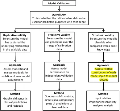
Model Validation

Overall Aim

To test whether the calibrated model can be used for predictive purposes with confidence

Structural validity

To ensure the model is plausible when compared with a priori

knowledge

Approach

Assess relative contribution of each model input to model

output

Method

Input relative importance; sensitivity

analyses analysis

Replicative validity

To ensure the model has captured the underlying relationship

in the available data

Approach

Assess model fit and analyse residuals for violation of error model

assumptions

Method

Graphical diagnostic plots of predictions

and residuals

Predictive validity

To ensure the model can generalise over the

range of calibration data

Approach

Assess model performance on independent validation

data

Method

Goodness-of-fit metrics; direct value comparison; plots of predictions vs

observed data

If an ANN model has been successful in approximating the relationship that is contained in the calibration data (i.e if the model is replicatively valid), the residuals should approximate the random error term, ˆ ≈. As such, if the above assumptions about are reasonable, these should also hold for ˆ

(Draper and Smith, 1998).

Violation of the LS assumptions may reveal deficiencies in the model. This could be due to an inappropriate model structure, such as insufficient model complexity, or the failure to find near-global optima in the error surface during calibration (training). Alternatively, the inability to approximate the desired relationship could be due to the absence of data on potential model inputs that have a significant impact on the model outputs, or the incorrect selection of model inputs from the available data. Consequently, when there is a discernible pattern in the residuals, attempts should be made to modify the model by re-visiting previous steps in the model development process, ensuring that appropriate model-development protocols are being followed (e.g., see Abrahart et al., 2008; Wu et al., 2014). In certain situations, how-ever, the LS assumptions may not be wholly plausible (e.g. in the case of heteroscedastic and/or autocorrelated measurement errors on y) and their violation may reflect the inappropriateness of the assumptions, rather than deficiencies in the model formulation (Clarke, 1973). In such cases, use of the SS criterion would result in invalid parameter estimates and inferences made about the process. Transformations, such as Box-Cox (Box and Cox, 1964), may be applied to the observed target data to correct for non-constant vari-ance and to improve the normality of the residuals (Bates and Watts, 1988), or alternatively, an alternative error model might be assumed for the pur-pose of calibration, which would result in more consistent model parameter estimates ˆθ (Sorooshian and Dracup, 1980; Kuczera, 1983; Thyer et al., 2009; Schoups and Vrugt, 2010; Evin et al., 2013). As a result, it is suggested that diagnostic checks be performed on the model residuals to determine whether the LS assumptions have been violated, and hence, whether any modifica-tions to the model or the error model are necessary to improve the replicative validity of the model.

2.2.2. Methods

is any non-random structure remaining in the model residuals:

• Scatter plot of observed versus predicted data. A scatter plot,

where paired observations and model predictions are plotted against each other, provides a simple method for graphically assessing how well the model fits the training data. For an accurate, unbiased model, the points should plot along the 1:1 line, with scatter about this line representing the discrepancy between the observations and the model. Visual inspection of this plot may reveal systematic divergence from the 1:1 line, which indicates unmodelled behaviour. The model may be shown to under- or over-estimate in a certain range if most points lie below or above the line. As such, a scatter plot is ideal for assessing model performance at low, medium, and high magnitudes (Bennett et al., 2013).

• Quantile-quantile (Q-Q) plot of observed versus predicted data.

Q-Q plots are powerful tools for graphically assessing goodness-of-fit and may be easier to interpret than scatter plots, especially if the num-ber of observations is either small or very large. To construct a Q-Q plot of the model predictions against the observations, these data sets are separately ranked, which removes the pairing between them, and the sorted predictions are plotted against the sorted observations. If the modelled and observed data are similarly distributed, points should plot approximately along the 1:1 line. Unlike the scatter plot, however, there should be no scatter about this line, since quantiles are plotted rather than paired data points. As a result, deviations from the line quickly reveal any differences in the distributions of modelled and ob-served data (e.g. biases at low or high magnitudes) (Chang and Hanna, 2004).

• Plot of observed and predicted data against data order. If

• Plot of standardised residuals against predicted data. This residual plot, with model output values on the x-axis and standard-ised residuals on the y-axis, is particularly useful for identifying non-constant variance in the residuals. Ideally, the residuals should display no pattern, plotting more or less in a horizontal band, symmetric about zero (if the residuals are normally distributed, 95% of the standardised residuals should lie between ±1.96). Non-constant variance, or het-eroscedasticity, is most commonly shown by a widening band, where there is as an increase in the variability of the residuals as the mag-nitude of the response increases (although it may also be shown by a narrowing band) (Bates and Watts, 1988). This plot can also be useful for identifying outliers in the data, which may indicated by particularly large residuals.

• Plot of standardised residuals against against order of the

data. If the spatial and/or temporal order of the data are known,

this plot may be useful for identifying serial correlation in the residu-als, which suggests unmodelled deterministic behaviour in the data. As above, there should ideally be no visible pattern in this residual plot and residuals should lie randomly within a horizontal band. However, if the residuals display positive serial correlation, sequences of residuals with the same sign will be present. On the other hand, negative serial correlation in the residuals may also be observed, where residuals of one sign tend to be followed by residuals of the opposite sign. If non-random structure is evident in this plot, the assumption of independent residuals and the use of the SS objective function for calibration may not be appropriate.

• Autocorrelation function (ACF) and partial-autocorrelation

function (PACF) plots. Similar to above, if the data are a time

series, the ACF and PACF plots (Box and Jenkins, 1976) can easily reveal if there is any autocorrelation in the residuals (such patterns may not be so easy to detect with a time series plot of the residuals). The ACF measures the autocorrelation in the residuals as a function of lag:

ACF =corr(ˆt,ˆt−k) (3)

ACF values (at lags greater than k = 0) lie within the 95% confidence bands around zero, given by ±1.96/√N. Significantly non-zero ACF values and a non-random pattern indicate that the residuals are serially correlated. The PACF measures the autocorrelation at lagk that is not accounted for by autocorrelations at shorter lags. While the PACF plot is not necessary for validating the model, if the ACF plot indicates correlated residuals, a time series model may be a more appropriate model for (e.g. t = φt−1 +zt where z ∼ N(0, σ2)) and the PACF

plot can be useful for identifying the order this model.

• Normal probability plot of residuals. A normal probability plot,

also known as a normal Q-Q plot, can be used to check whether the residuals are consistent with a Gaussian distribution (i.e. whether the normality assumption is reasonable). This plot is constructed by plot-ting sorted values of the standardised residuals against the correspond-ing theoretical values from the standard normal distribution. If the residuals are normally distributed, they will plot along, or close to, a straight line. Departure from this straight line indicate that the resid-uals are probably not consistent with the Gaussian distribution. Addi-tionally, the normal probability plot may indicate how the distribution differs from normal: significant deviations at the end of the line may indicate the presence of outliers, while curvature can indicate skewness or long tails (Heiberger and Holland, 2004).

• Histogram of residuals. A histogram of the residuals also allows for

the normality of the residuals to be graphically checked. However, it is helpful to view such a plot in addition to the normal probability plot, as a histogram gives a clearer picture of the shape of the residual dis-tribution, providing a graphical summary of the shape, scale, location and symmetry (or lack thereof) of the residuals. The normal proba-bility plot, on the other hand, allows for easier detection of deviations from the normal distribution.

Examples of these plots are shown and discussed in Section 5.

2.3. Predictive Validation 2.3.1. Underlying philosophy

- the calibration data (Chapra, 1997). However, good performance of the model over the calibration data set does not guarantee correct predictive behaviour of the model (Power, 1993). This is because the calibration data might not be representative of the available data or the model might have been overfitted to the calibration data, thereby “learning” the specific pat-terns in the calibration data, rather than the general underlying relationship. Consequently, the purpose of predictive validation is to check whether the model can generalize over the range of the data used for calibration (Fig. 1). In order to achieve this, the predictive performance of the model is checked on a dataset that was not used during calibration or any other part of the model development process (Maier et al., 2010). Care needs to be taken that the validation data are representative of the data used for calibration, which can be achieved using a range of data splitting methods (May et al., 2010; Wu et al., 2013).

2.3.2. Methods

metrics are listed in Table A.1, along with a brief description. For a more detailed explanation of these metrics readers are referred to Dawson et al. (2007, 2010); Bennett et al. (2013).

In addition to the metrics given in Table A.1, it is suggested that sum-mary statistics of the observed and predicted datasets, including the mean, minimum, maximum, variance, standard deviation, skewness and kurtosis, be compared (these statistics are also returned by HydroTest). A compari-son of such statistics between the observed and predicted data sets allows a ‘direct value comparison’, whereby the characteristics of the predicted and observed data sets are compared as a whole, rather than on a point-by-point basis (Bennett et al., 2013). Ideally, the summary statistics computed for the model predictions should be very close in value to those computed based on the observations; however, a direct value comparison can be particularly useful for quickly identifying how the predictions might differ from the ob-servations, which will not be obvious from the goodness-of-fit metrics given in Table A.1. Furthermore, the metrics in Table A.1 return a single value for the whole dataset, which can disguise significant divergent behaviour over time or space (Bennett et al., 2013). As such, it is also recommended that the first three plots described in Section 2.2.2 (scatter plot, Q-Q plot and plot of observed and predicted data versus data order) be constructed for the validation data, since these plots may provide valuable insights about the way a model performs that will not be evident from an assessment of such single-value metrics.

2.4. Structural Validation 2.4.1. Underlying philosophy

has been identified, it is helpful for identifying models that are not plausible from a physical perspective.

2.4.2. Methods

Given the interconnected nature of ANN nodes and the nonlinear trans-fers applied within them, ANN connection weights are typically much less interpretable than the parameters of more traditional statistical models and, as such, provide little insight into the internal behaviour of an ANN model. In environmental modelling studies, efforts to extract the ‘knowledge’ em-bedded within a trained ANN have typically been aimed at quantifying the strength of the relationships between individual inputs and the output or at understanding the relationships represented by the hidden nodes. The latter approach is based on the idea that different physical sub-processes may be represented by individual hidden nodes (e.g., see Wilby et al., 2003; Jain et al., 2004; Sudheer and Jain, 2004; See et al., 2008; Jain and Ku-mar, 2009). However, due to the distributed nature of ANNs, individual hidden nodes generally do not correspond well with features in the problem domain. Rather, these physical components are likely to be encoded across a number of hidden nodes, and similarly, each hidden node may partially rep-resent a number of different system components (Craven and Shavlik, 1997). Consequently, it may be difficult, in general, to structurally validate ANN models using these methods. The former approach includes different sensi-tivity analysis (SA) methods, whereby the effects of variation of the inputs on the output are assessed (Maier et al., 1998; Abrahart et al., 2001; Shahin et al., 2005; Sudheer, 2005; Park et al., 2007; Mount et al., 2013; Dawson et al., 2014), as well as methods based on the examination of the connection weights themselves (Olden and Jackson, 2002; Gevrey et al., 2003; Olden et al., 2004; Kingston et al., 2005b, 2006b; Jain et al., 2008).

(i.e. certain methods may appear to be more accurate than others depending on the complexity - nonlinearity, monotonicity, variable interdependency and interactions, etc. - of the comparison data), making it difficult to reach a consensus on which method, if any, is the best for quantifying input RI. Sarle (2000) presents a useful discussion on the limitations of various methods for quantifying input RI and how some methods may be more accurate in certain situations than others. Based on this discussion, together with the results of the aforementioned comparison studies, five methods, namely Garson’s, the Connection Weight (CW), modified CW (MCW), Profile and Partial deriva-tives (PaD) methods, are suggested for assessing the structural validity of calibrated ANN models as part of the proposed validation framework. The first three methods directly use the connection weights to compute input RI, while the last two methods are SA approaches that examine the change in the model output as a result of input variation. These methods are described briefly below while further details, including the advantages and limitations of the methods, are provided in Appendix B.

1. Garson’s method: Garson’s algorithm (Garson, 1991), or the ‘Weights’

method as it was called in the comparison carried out by Gevrey et al. (2003), was one of the earliest methods proposed for quantifying the RI of ANN inputs based on the connection weights and has been used in numerous environmental modelling studies for extracting information from trained ANNs (Brosse et al., 1999; Abdul-Wahab and Al-Alawi, 2002; Mi et al., 2005; Jain et al., 2008; Langella et al., 2010; Sreekanth and Datta, 2010; Phukoetphim et al., 2014; Kumar, 2014; Coad et al., 2014; Beck et al., 2014). Using this method, input RI is calculated by partitioning the hidden-output layer connection weights into com-ponents associated with each input node using absolute values of the connection weights. Since absolute values of the weights are used, it is only possible to estimate the magnitude but not the direction of the input contributions (i.e. whether an input has a positive or negative effect on the output).

2. CW method: The CW approach of Olden and Jackson (2002) was

and Worner, 2008; Watts et al., 2011; Beck et al., 2013; Sun, 2013). Using this approach, RI is computed based on an ‘overall connection weight’ between each input and the output, which in turn, is based on products of input-hidden and hidden-output connection weights for each input summed across all hidden nodes. In this approach, raw rather than absolute values of the weights are used, making it possible to estimate both the magnitude and direction of the input contribu-tions.

3. MCW method: Kingston et al. (2006a, 2010) introduced a

modi-fied CW method, where input RI is computed in the same fashion as the CW approach; however, the raw input-hidden node weights are “squashed” using the hidden layer activation functions. In comparison to the CW approach, this method has been shown to provide improved estimates of input RI in certain situations (Kingston et al., 2010).

4. Profile method: The Profile SA method, first described in Lek et al.

(1995, 1996), involves successively varying each input variable across its range while keeping all others constant at their minimum, first quar-tile, median, third quarquar-tile, and maximum values; thus, producing five output profiles displaying variation in the output over the range of the input variable of interest. The median predicted responses across the five output profiles is also calculated, from which it is possible to assess the median behaviour of the model, given a range of different input values. In addition, the RI of each input is calculated based on the magnitude of the range of median output values produced by varying each input. Being relatively quick and easy to apply, SA methods have been popular for investigating input contributions in ANNs used for en-vironmental modelling applications (e.g., see Maier et al., 1998; ¨Ozesmi and ¨Ozesmi, 1999; Liong et al., 2000; Shahin et al., 2005; Young Ii et al., 2011).

5. PaD method: The PaD method (Dimopoulos et al., 1995, 1999) is

mod-elling studies to quantify ANN input variable contributions Park and Chung (2006); Park et al. (2007); Tison et al. (2007); Vasilakos et al. (2008); Laffaille et al. (2009); Olaya-Mar´ın et al. (2012); Kumar (2012). Similar to the Profile method, this approach returns a profile of partial derivatives for each ANN input, which can be interpreted in a similar way to the coefficients in linear models, as well as a measure of input RI for each input.

3. R-Package for Implementing Proposed Validation Framework

A toolbox for implementing the proposed validation framework is avail-able in the validann package, which has been developed for the R software environment (R Core Team, 2015) and is available from the Comprehensive R Archive Network (CRAN) at http://CRAN.R-project.org/package=validann. The R environment was chosen as the development platform for this toolbox for a number of reasons. Firstly, it is free, open source and runs on all major platforms. Secondly, its package system allows for the simple distribution, use and maintenance of third-party code. Finally, a user’s ability to add functions and write scripts in R facilitates the extension and adaptation of the function-ality provided by the standard R environment and its many add-in packages. As such, thevalidannR package should not only enable researchers to read-ily access the proposed ANN validation methods, but also to manipulate and adapt these methods as required in order to integrate them into their own work; thus encouraging their maximum uptake and use. While there are al-ready methods and packages available within the R environment that can be used to perform many of the validation tests recommended within the pro-posed validation framework (e.g. hydroGOF (Zambrano-Bigiarini, 2014) for computing and plotting goodness-of-fit measures between observed and simulated values, NeuralNetTools (Beck, 2015) for performing sensitivity analyses and computing ANN input importance measures, and indeed many of the other statistical and plotting methods available in the pre-installed R base packages), the validann package expands upon these methods and combines them into a single validation package that can be easily applied for consistent and comprehensive validation of ANN models developed both within and outside of the R environment.

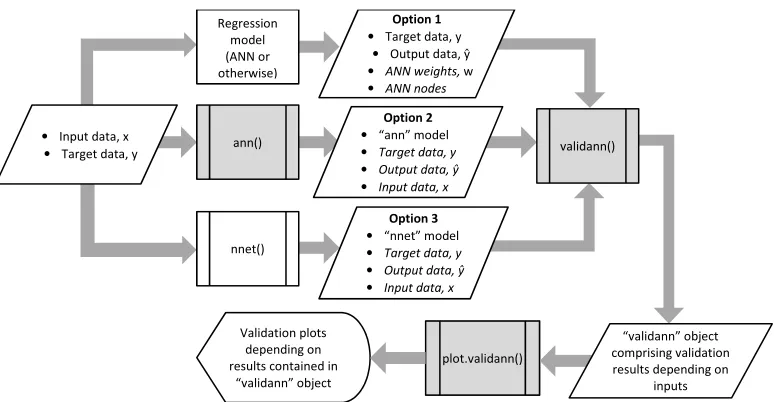
As shown in Fig. 2, the validann package has three core functions. The

plot.validann() Regression

model (ANN or otherwise)

Option 2 • “ann” model

• Target data, y

• Output data, ŷ

• Input data, x

• Input data, x • Target data, y

Option 3 • “nnet” model

• Target data, y

• Output data, ŷ

• Input data, x

nnet()

ann() validann()

Option 1 • Target data, y

• Output data, ŷ

• ANN weights, w

• ANN nodes

“validann” object comprising validation results depending on

inputs Validation plots

depending on results contained in

“validann” object

Figure 2: Structure and core functions (shaded grey) of validannR-package. Italics are used to denote optional inputs to the functions.

replicative, predictive and structural validation metrics associated with the proposed validation framework, as outlined in Section 2, and to present the results in a user-friendly and efficient manner. In addition, the package includes the ann() function for constructing ANN models. These functions are described in further detail below.

Essential arguments to theann()function are the input (x) and target (y) training data and the number of hidden layer nodes. By default, the method uses a logistic sigmoid activation function for the hidden layer nodes and a linear activation at the output layer. The default objective function is the sum of squared residuals as defined by Eq. 2 and training is performed using the built-inoptim()R function with the Broyden-Fletcher-Goldfarb-Shanno (BFGS) method, a quasi-Newton gradient-based optimisation method, as a default (although any of the optim() methods may be selected if appro-priate). Once a fitted ANN model has been obtained using ann(), other standard R methods are provided to work with the ‘ann’ objects returned. These include predict() to predict model outputs using a trained ANN and new input data, as well as fitted(), observed() and residuals()to extract the training outputs, targets and model residuals, respectively.

Function validann() is the foundation of the validann package. This generic function computes all of the validation metrics and statistics discussed in Section 2 according to the class of ANN model (if supplied) and the data provided. There are three main options for using this function, as shown in Fig. 2, where italics are used to denote optional inputs to the functions. The first option (Option 1 in Fig. 2) takes observed target data and simulated model outputs as inputs and returns goodness-of-fit metrics, model residuals and statistics related to the distribution of the residuals and the observed and simulated data. Additionally, if the weights of a trained ANN are supplied together with the numbers of nodes in each layer, input relative importance measures computed using Garson’s method and the CW method will be returned. However, since this option only allows for limited information regarding the internal dynamics of the model to be provided, additional structural validation metrics cannot be computed. As such, this option is the least preferred, as it only allows for limited structural validation of the model. However, it is also the most general option and may be useful in cases where the ANN model has been built outside of the R environment and/or is not of class ‘ann’ or ‘nnet’ (or indeed is not even an ANN). It may also be useful for predictive validation, once replicative and structural validation metrics have already been computed using either Options 2 or 3 in Fig. 2, as discussed below.

returned by the ann() function. Additionally, both the Profile and PaD methods will only be carried out if the input data used for training are supplied. Output and target data are only optional inputs using this option, since if they are not supplied, the output and target data stored in the ‘ann’ object will be used for computing goodness-of-fit metrics, residuals and data summary statistics. This may be sufficient for replicative validation; however, for predictive validation, observed and simulated data for an independent validation set must be supplied.

The third option for calling thevalidann()function (Option 3 in Fig. 2) allows for validation of ANN models of class ‘nnet’ built using the nnet()

function from package nnet. Given the same inputs, this option will return the same results as Option 2, with the exception of the PaD results, as the hidden and output node partial derivatives required by this method are not returned by the nnet() function. As with Option 2, the output and target data are optional inputs (since corresponding data stored in the ‘nnet’ object may be used); however, for predictive validation, these data must be supplied. It is important to note that, regardless of which option is chosen, the

validann() function must be called twice in order to produce results for predictive and replicative validation: once with the training data, and ideally the ANN weights and model structure, as inputs (replicative and structural validation) and then again using the independent validation data (predictive validation). All three of the options return a list object of class ‘validann’ which includes components according to the inputs supplied when calling the

validann() function. At most (i.e. when the ANN model is of class ‘ann’ and input data are included in the function call), a ‘validann’ object will be comprised of the components given in Table 1.

Finally, the plot.validann() function is a plot method for objects of class ‘validann’ that produces a series of plots according to the components of the validann object supplied. By default, the plots produced are grouped into goodness-of-fit, residual analysis and sensitivity analysis plots, with mul-tiple plots to a page, as follows:

• Goodness-of-fit plots (predictive, replicative validation): scatter and Q-Q plots of observed versus predicted data and observed and predicted data against data order.

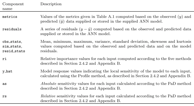
au-Table 1: Components of avalidannobject.

Component name

Description

metrics Values of the metrics given in Table A.1 computed based on the observed (y) and predicted (ˆy) data supplied or stored in the supplied ANN model.

residuals A series of residuals (y−yˆ) computed based on the observed and predicted data supplied or stored in the ANN model.

obs stats,

sim stats,

resid stats

Mean, minimum, maximum, variance, standard deviation, skewness and kurtosis values computed based on the observed and predicted data and on the model residuals.

ri Relative importance values for each input computed according to the five methods described in Section 2.4.2 and Appendix B.

y hat Model response values indicating the local sensitivity of the model to each input, calculated using the Profile method, as described in Section 2.4.2 and Appendix B.

as Absolutesensitivity values for each input calculated according to the PaD method described in Section 2.4.2 and Appendix B.

rs Relativesensitivity values for each input calculated according to the PaD method described in Section 2.4.2 and Appendix B.

tocorrelation plots; standardised residuals against predicted data and standardised residuals against against order of the data.

• Sensitivity analysis plots (structural validation): Profile sensitivity plots: for each input, plots of predicted response versus percentile of input; PaD sensitivity plots: for each input, plots of relative and absolute sensitivity versus observed response.

have not been populated). If the plot device is interactive (i.e. the screen), the user is prompted to view the next plot or group of plots. However, if another graphics device is specified (e.g. jpeg, postscript, pdf), all plots will be displayed in a single file. The style and format of the plots produced by the plot.validann() function are not easily manipulated; however, all val-idation results used in the creation of the plots are stored in the ‘validann’ object returned by function validann(), giving users the ability to create their own validation plots as desired.

4. Case Studies

The proposed ANN validation framework was applied to two real en-vironmental modelling case studies in order to demonstrate the benefits of considering replicative and structural validity in addition to predictive valid-ity. Since not all of the proposed framework methods are suited to all types of problems, the case studies were selected to demonstrate the framework when applied to two problems that are fundamentally different in nature: (i) a forecasting problem with strong temporal dependencies and highly corre-lated inputs and (ii) a prediction problem with no temporal component and relatively independent inputs. The results of these case studies, presented in Section 5, also demonstrate the types of outputs generated by the core functions of the R-package validann.

4.1. Background and Data

4.1.1. River Murray (Australia) salinity forecasting

et al., 2005; Kingston et al., 2005b, 2008; Fernando et al., 2009). To deter-mine the important inputs for forecasting Murray Bridge salinity 14 days in advance, Fernando et al. (2009) used a partial mutual information (PMI) approach to select from a total of 1304 candidate inputs (including lags of up to 113 days for each of the 16 candidate input variables). They found three inputs to be significant: Waikerie salinity (WAS), Mannum salinity (MAS) and flow at Lock 7 (L7F), each a time lag of one day (t−1).

In line with previous studies, variables WASt−1, MASt−1 and L7Ft−1were

used as inputs for forecasting Murray Bridge salinity 14 days in advance (MBSt+13), with data between December 1986 and June 1992 used for

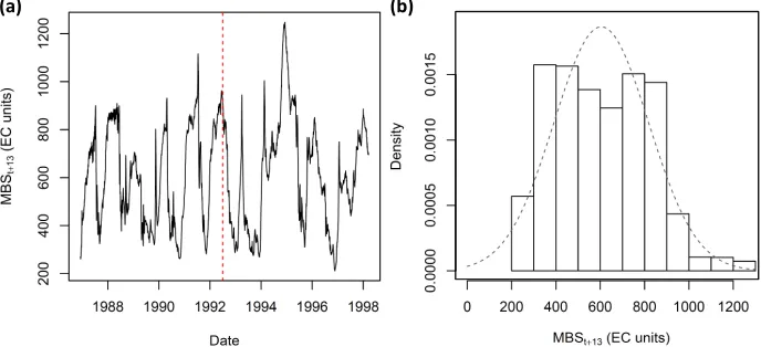
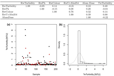
train-ing and data from July 1992 to April 1998 used for independent validation. A time series plot of the target MBSt+13 data is shown in Fig. 3 (a), where

data to the left of the red dashed line are the training targets, while those to the right of the line are the validation targets. In Fig. 3 (b), a histogram of the MBSt+13 data shows that the distribution of these data is reasonably

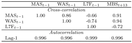
normal. In Table 2, it can be seen that the upstream salinity and flow inputs for this forecasting problem are moderately to highly correlated with one an-other and with the target salinity concentration at Murray Bridge, and each input and the output are highly autocorrelated.

(a) (b)

Figure 3: (a) Time series of MBSt+13 data. The red dashed line denotes the split between

training and validation data; training data are to the left and validation data to the right. (b) Histogram of the MBSt+13 data. The grey dashed line denotes the Gaussian

Table 2: River Murray salinity data cross- and autocorrelation coefficients

MASt−1 WASt−1 L7Ft−1 MBSt+13

Cross-correlation

MASt−1 1.00 0.86 -0.66 0.91

WASt−1 1.00 -0.74 0.94

L7Ft−1 1.00 -0.72

Autocorrelation

Lag-1 0.996 0.996 0.999 0.996

4.1.2. Surface water turbidity prediction, Australia

The southern Australian turbidity (SAT) dataset has previously been studied by van Leeuwen et al. (1999) and Maier et al. (2004) who developed ANN models to assist treatment plant operators with determining optimal alum doses for water treatment plants in southern Australia. In addition, the dataset has subsequently been used by Wu et al. (2013) for comparing the performance of different data splitting methods used in the development of ANN models.

The SAT dataset, as discussed in Maier et al. (2004), comprises 202 mea-surements of raw and treated water quality parameters including turbidity, pH, colour, ultraviolet absorbance at a wavelength of 254 nm (UVA-254), al-kalinity and dissolved organic carbon (DOC), together with the correspond-ing alum doses. Raw water parameters were collated from 29 raw water samples collected from 14 different surface water sources located in southern Australia. The corresponding treated water quality parameters were mea-sured from jar tests, where each of the raw water samples was dosed with a number of different alum concentrations and the resulting water quality parameters were recorded. Wu et al. (2013) used a PMI approach to se-lect the relevant inputs for predicting treated water turbidity (TwTurbidity) from the six raw water quality parameters (RwTurbidity, RwPh, RwColour, RwUvAbs254, RwAlkalinity and RwDOC) and the alum dose, finding Rw-Turbidity, RwPh, RwColour, RwUvAbs254 and the alum dose to be signif-icant. They then used four data splitting methods to divide the available data into training (60%), testing (20%) and validation (20%) datasets.

Table 3: SAT dataset cross-correlation coefficients

RwTurbidity RwPh RwColour RwUvAbs254 Alum Dose TwTurbidity RwTurbidity 1.00 -0.05 0.14 -0.21 0.10 0.40

RwPh 1.00 -0.15 0.08 0.20 -0.01

RwColour 1.00 0.76 0.32 0.14

RwUvAbs254 1.00 0.39 0.00

AlumDose 1.00 -0.22

(a) (b)

(NTU)

(N

T

U

)

Figure 4: (a) SAT target TwTurbidity data. Black dots denote the training data; red dots denote the validation data. (b) Histogram of the TwTurbidity data. The grey dashed line denotes the Gaussian distribution.

4.2. ANN Model Development and Validation

For each case study, 15 different ANN structures were considered with the number of hidden nodes increasing from 1 to 15. Additionally, for each of the 15 network structures, the connection and bias weights were initialised five times with different random starting values between -0.1 and 0.1, re-sulting in a total of 75 ANN models being developed for each case study. All ANNs were single hidden layer networks with hyperbolic tangent (tanh) hidden layer activations and a linear activation at the output. All input data were standardised to have a mean of zero and standard deviation of one, while the target data were linearly rescaled between 0 and 1. The models were built in R (3.2.2) using the ann() function from the validann pack-age discussed in Section 3, with the default BFGS optimisation algorithm used for training. All models were trained without cross-validation or early stopping for a maximum of 500 iterations using the default sum of squared residuals as an objective function.

To validate the models, thevalidann()function from thevalidann pack-age was applied twice to each model: the first time using the (unscaled) training data to obtain replicative and structural validation results, and the second time using the (unscaled) independent validation dataset to obtain predictive validation results. Three of the best performing models, in terms of predictive validity, were selected from each case study and used to compare and contrast the corresponding replicative and structural results.

5. Results and Discussion

5.1. River Murray salinity forecasting

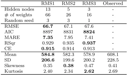
good summary of how well the model fits the data over a range of different magnitudes (low, average and high), as well as a comparison between the model fit and model complexity. Moreover, they are applicable to data with or without a time component and, consequently, are also suitable for assess-ing the performance of the turbidity case study models. As can be seen in Table 4, all three models give a good fit to the validation data (CE≥ 0.9), with relatively little difference in their predictive performance, particularly considering the large variation in the size of the three models. As can also be seen, there is no definitive “best” model in terms of the performance metrics or summary statistics presented. Rather, model RMS1 with 13 hidden nodes appears to give the best overall fit to the data, while model RMS3 with three hidden nodes is the most parsimonious, providing a comparable fit to the data with significantly fewer weights (free parameters). Model RMS2 sits between these other models, achieving a slightly better fit to the data than RMS3, but still with many fewer weights than RMS1.

Table 4: River Murray salinity predictive validation results. Best results are highlighted in bold text.

RMS1 RMS2 RMS3 Observed Hidden nodes 13 5 3 -# of weights 66 26 16

-Random seed 3 3 1

-RMSE 66.7 67.1 67.6 -AIC 8897 8831 8824 -MARE 7.35 7.95 7.41 -RSqr 0.929 0.935 0.937

-CE 0.915 0.914 0.913

-Mean 584.8 582.3 578.9 608.1

SD 206.6 199.6 200.2 228.5

Skewness 0.35 0.38 0.47 0.41 Kurtosis 2.40 2.34 2.62 2.69

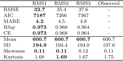
Model performance results for models RMS1, RMS2 and RMS3 when ap-plied to the training data (replicative validity) are given in Table 5. These results are similar to the predictive validation results presented in Table 4, in that an improved fit to the data is achieved as the number of parameters is in-creased. This is not surprising, since no early stopping to prevent overfitting was applied. However, when applied to the training data, the best (smallest) AIC value was also obtained using the largest model (RMS1), suggesting the extra complexity of this model is warranted given the superior fit achieved.

(a) (b)

(c) (d)

(e) (f)

Table 5: River Murray salinity replicative validation results. Best results are highlighted in bold text.

RMS1 RMS2 RMS3 Observed RMSE 32.7 35.4 37.6 -AIC 7187 7266 7367 -MARE 4.2 4.5 4.8

-RSqr 0.973 0.968 0.964

-CE 0.973 0.968 0.964

-Mean 600.7 600.7 600.7 600.7

SD 194.9 194.4 194.0 197.6

Skewness 0.11 0.11 0.12 0.11 Kurtosis 1.68 1.69 1.67 1.75

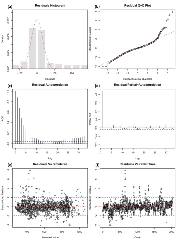
and validation datasets. However, the results of the residuals analysis for this model, presented in Fig. 5, show that the residuals are strongly autocor-related, as indicated by the ACF plot in Fig. 5(c), where the majority of lags show significant autocorrelation (ACF values outside of the 95% confidence bands). In fact, similar results were observed for all three models RMS1, RMS2 and RMS3 (although not shown here for the purpose of brevity), indicating a possible deficiency in the models, which might be due to the omission of important input information. Ideally, in such circumstances, the model development steps should be revisited, including the selection of model inputs. However, reselection of model inputs was beyond the scope of this pa-per and the following autoregressive error model with lag-2 autocorrelations (AR(2)) was instead assumed in the attempt to account for any predictable component remaining in the residuals:

t=φ1t−1+φ2t−2+zt; zt ∼N(0, σz2) (4)

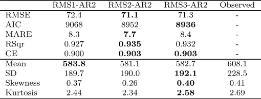
The order of this error model was selected according to the number of lags displaying significant autocorrelation in the PACF plot shown in Fig. 5(d). The models were retrained using the new error model and residual analysis methods were subsequently applied to the innovations, z, rather than the raw residuals, in order to test the replicative validity of the three new models RMS1-AR2, RMS2-AR2 and RMS3-AR2.

As can be seen in Fig. 6, the autocorrelation was reasonably well captured by the error model given by Eq. 4 for all three models, since the ACF of the innovations, zt, at lags ≥ 1 are mostly within the 95% confidence bands

refer-ence to the predictive validation results presented in Table 6, it can be seen that, although a slightly inferior fit to the validation data was achieved using an AR(2) error model than the standard SS residuals objective function, a good fit (CE ≥ 0.9) to these data was still achieved by all three models. In this case, the RMS2-AR2 and RMS3-AR2 models appear to be the most predictively valid according to the metrics and statistics presented in Table 6.

0 5 10 15 20 25 30 Lag

0 5 10 15 20 25 30 Lag

0 5 10 15 20 25 30 Lag

A

C

F

0

.0

0

.2

0

.4

0

.6

0

.8

1

.0

(a) RMS1-AR2 (b) RMS2-AR2 (c) RMS3-AR2

Figure 6: ACF plots obtained using models (a) RMS1-AR2, (b) RMS2-AR2 and (c) RMS3-AR2. Blue dashed lines denote the 95% confidence bands around zero.

Table 6: Predictive validation results for models RMS1-AR2, RMS2-AR2 and RMS3-AR2. Best results are highlighted in bold text.

RMS1-AR2 RMS2-AR2 RMS3-AR2 Observed

RMSE 72.4 71.1 71.3

-AIC 9068 8952 8936

-MARE 8.3 7.7 8.4

-RSqr 0.927 0.935 0.932

-CE 0.900 0.903 0.903

-Mean 583.8 581.1 582.7 608.1

SD 189.7 190.0 192.1 228.5 Skewness 0.37 0.26 0.40 0.41 Kurtosis 2.44 2.34 2.58 2.69

Using the PMI input selection procedure, Fernando et al. (2009) found that the order of importance of the selected RMS inputs, from most impor-tant to least, was WASt−1, MASt−1 then L7Ft−1. This finding is supported

by the scatterplot of RMS model inputs versus MBSt+13presented in Fig. 7,

where it can be seen that there is strong, positive correlation between the output MBSt+13and inputs WASt−1 and MASt−1, with the WASt−1-MBSt+13

●● ● ● ●●● ● ● ●● ● ●●●● ● ●● ● ● ● ● ● ●●●●●●● ● ● ● ● ● ● ● ● ● ●●●●●●●● ●●● ●●●●●● ●●●●●● ●● ● ●●●● ● ● ● ●●●●●●●●●●●● ● ● ●●●● ●●●●●●●●●●●● ●● ● ● ●● ●● ●●●●● ● ●● ●● ●●●●● ● ● ● ● ● ● ● ●●●●●●●●●● ●●●● ● ● ●●●●●●●●● ●●●●●● ● ●● ● ● ●●● ● ● ●●● ●●●●●●●● ● ● ● ● ● ●● ●●●●● ● ● ●●●●●●●●●●●● ● ●●●●● ●● ● ● ● ● ● ● ● ● ● ● ● ● ● ● ● ● ● ● ● ● ● ● ● ● ● ● ● ● ● ● ● ● ● ● ● ● ● ● ● ● ●● ● ● ● ● ● ● ● ● ● ● ● ● ● ● ● ●●● ●●● ● ●●●●● ● ●●●●● ●●●●●●●● ● ● ●●●● ●●●● ●●●●●●●●●●● ● ●●●●● ● ● ●●●●● ● ● ●●●●● ●●●●●●●●●●● ●●● ●● ● ● ● ●● ● ● ● ●●●●●● ●●●●● ● ● ●●●●● ● ● ● ●●● ● ●●●● ●●●●● ●●●●●●●●●●●●●● ●●●●●●●● ● ● ●●● ●●●●●●●● ● ● ● ●● ● ● ●●●● ●●●●●●● ●●●●●●●●● ● ● ● ● ● ●● ● ●●●●●●●●●● ● ●●●● ●●●●● ● ●●●●●● ● ● ●●●● ● ● ● ● ● ● ● ● ●●●●●●●● ● ● ●● ●●● ●● ● ● ● ●●● ● ● ● ● ● ● ●●● ●●●●●●● ●●●●●●● ● ● ● ● ● ● ● ● ● ● ● ● ● ● ● ● ● ● ● ● ● ● ● ● ● ● ● ● ● ● ●● ● ●●● ●● ●●● ● ● ● ● ● ●●●●●●● ●● ● ● ● ● ● ● ● ● ● ● ● ● ● ● ● ● ● ● ● ● ● ● ● ● ● ● ● ● ● ●● ● ● ● ● ● ● ● ● ● ● ● ● ● ● ● ● ● ● ● ● ● ● ● ● ● ● ● ● ● ● ● ● ● ● ● ● ●●● ● ● ● ● ●●●●●●●●●●●● ●●● ●● ●● ● ● ●●● ●●● ●● ● ● ● ● ● ● ● ● ● ● ● ● ● ●●●●●● ●●● ●●●●●●●●●●●●●●●●●●● ●●●●●●●●●●● ● ●●●●●●●●●●●● ● ● ● ● ● ●●● ●●●●●● ● ● ● ● ● ● ● ● ● ● ● ● ●●●● ●●●●●●●●●● ● ● ● ● ● ● ●●●●●● ● ● ● ●●●●●● ●●●●●●●●●●●● ●● ● ● ● ● ● ● ● ● ● ● ● ● ● ● ● ● ● ● ● ● ● ● ● ● ● ● ● ●● ● ● ● ● ● ● ● ● ● ● ● ● ● ●● ● ● ●● ● ● ● ●●●●● ● ● ● ● ● ● ●●●●●●●●●●●●● ● ● ●●●●● ● ● ● ● ● ●●●●● ●●●● ●●●● ● ● ● ● ● ● ● ● ● ●●●●●● ● ● ● ● ● ● ● ● ● ●●●●●●● ● ●●●●●● ●●●●●●● ● ●●●●●●●●●●●●● ● ● ● ● ● ● ● ● ● ● ● ● ● ● ● ● ● ● ● ● ● ● ● ● ● ● ● ● ● ● ● ● ● ● ● ● ● ● ● ● ● ● ● ●●●●●●● ● ●● ● ● ● ● ● ● ● ● ● ●● ● ● ● ● ● ● ● ● ● ● ● ● ● ● ● ● ● ● ● ● ● ● ●●●● ●● ●● ●●●●●●●●●●●●●● ●●●● ●●●●●●●● ●●● ● ● ●●● ●●●●● ●●●● ●●●●●● ● ● ● ● ● ●●●●●● ●●●●●●●●●● ●●●●●●● ●●●●●●●● ●●●●● ●●●●● ● ● ● ● ●●●●●●●●●●●●●●●●●●● ●●●● ●● ● ●●●●●●●● ● ● ● ● ● ● ● ● ● ● ● ● ● ● ● ● ● ● ● ●● ● ● ● ● ● ● ● ●●●●● ● ● ● ● ● ● ● ● ● ● ● ● ●●● ● ●●● ● ●● ● ● ●●●●● ●●●●●●●●● ● ●●● ● ● ● ● ● ● ● ●●● ● ● ● ●●● ● ● ● ● ● ● ● ● ● ● ● ● ● ● ● ● ● ● ● ● ● ● ● ● ● ● ● ● ● ● ● ● ● ● ● ● ●● ● ●● ● ● ● ● ●●●●●●●●●● ●●●●●●●●● ● ● ● ● ● ● ● ● ● ● ● ● ● ● ● ● ● ● ●●●●●● ● ● ● ●●●●●●●●●●●●●●●●●● ● ●●● ● ● ●●● ●●● ●● ●●●●●● ● ●● ●●●●●●●●●●●●●●●●●●● ●●●●●● ●● ●●●● ●● ●●●●●● ●●●● ●● ●●●● ●●●●●●●●●●●●●● ● ● ● ● ● ● ●●●●●●●●●●●●●●●●●●● ● ●● ● ● ● ● ●● ●●●●●●●●●●●● ● ● ● ●● ● ● ● ●●●●●●●●●●●●●● ● ●●● ● ● ●●● ● ● ● ● ●●●● ●●●● ● ●● ● ● ●● ●●●●●●●●●● ●● ● ● ● ● ●●●●●●●●●●●●●●●●● ● ● ● ● ● ● ● ● ●●●●●●●●● ●●●●● ● ●● ●●●●●● ● ● ● ● ● ● ● ● ● ● ● ● ● ● ● ● ● ● ● ● ● ● ●●●●● ● ● ● ●● ● ● ● ● ● ● ● ● ● ● ● ● ● ● ● ● ● ● ●● ● ● ● ● ● ● ● ● ● ● ● ● ● ● ● ● ● ● ● ● ● ● ● ●● ● ● ●●●● ● ● ● ● ● ● ● ● ● ● ● ● ● ● ● ● ● ● ● ● ●●●● ● ● ● ● ● ● ●●●●●●●●●●●● ● ● ●●● ● ●●● ●●●●●●●● ● ● ●● ●●● ●●●●● ● ●●● ●● ● ● ● ● ● ● ●● ●●●●●●●●●●●● ● ●●●●● ● ● ● ●●●●● ● ● ●●●●●●●●●● ●● ●●●●●●●●●●●●●●●●●●●●●●●●●●●●●●●●● ● ● ● ● ● ● ● ● ●●●●● ● ● ● ● ●● ●●●●● ● ●● ●●●●● ●●●● ● ● ●●●●●●● ●●●●●●●●●●●●●● ●●●●●●●●●●●●● ●●●●●●●●●●●●● ●●●●●●●●●

400 600 800 1000

400

600

800

1000

MBSt+13 (EC units)

Salinity (EC units)

●● ● ● ●●●●● ● ● ● ●●● ●● ● ● ●●●●● ● ●● ● ●●● ● ● ● ● ● ● ● ●●●● ● ● ● ●●●● ●● ●●●●● ●● ●●● ●● ●● ●● ● ●● ●●● ●●●●●●● ● ● ● ● ● ● ● ●●●● ●●●●●●●●●● ● ●●●●● ●● ● ●●● ● ● ● ● ●●●●●●●●●● ● ● ● ● ● ● ●● ●●●●●● ● ● ●●●● ● ● ●●●●●●●●●●●●●●● ●●●●●●●● ● ● ●● ●● ● ● ● ● ● ●●● ●● ●● ● ●●●●●●●●●●●●●●●●●●● ● ● ● ●●●● ●● ● ● ● ● ● ● ● ● ● ● ● ● ● ● ● ● ● ● ● ● ● ● ● ● ● ● ● ● ● ● ● ● ● ● ● ● ●●●● ● ● ● ● ● ● ● ● ●● ● ● ● ● ● ● ● ● ● ● ● ● ●● ●● ●● ●●●● ●●●● ●● ●●●●●● ● ●●●●● ● ● ● ● ●● ● ● ● ●● ●● ● ● ●●●●●● ● ●● ●● ● ● ●●●●●●● ● ● ●●●●●●●●●● ● ●● ● ● ● ●●●● ● ●●_{● ●} ● ● ●●●●●● ●●●● ●● ● ● ● _●● ● ● ●●●●●●●●●●●●●●●● ●●●●● ● ●●●●●● ●● ● ● ● ●●● ●●●●●●●●● ● ● ●●●● ●●●● ●●●●●●● ●●●●●●●● ● ● ● ● ● ● ●● ● ●●●●●● ●●● ● ● ●●●● ●●●●● ● ●●●● ● ●●●●●●●●●●●●● ●● ●● ● ● ● ● ● ● ● ● ●● ● ● ● ●● ● ● ●●●●●●●● ● ● ●●●●●●●● ● ● ● ● ● ● ● ● ● ● ● ● ● ●● ● ● ● ● ● ●● ● ● ● ● ● ● ● ● ● ● ● ●●● ● ● ● ●●●● ●● ●● ● ● ● ● ● ● ● ● ●●●●●●● ● ● ● ● ● ● ● ● ● ● ● ● ● ● ● ● ● ● ● ● ● ● ● ● ● ● ● ● ●●●●● ● ●● ● ● ● ● ● ● ● ● ● ● ● ● ● ● ● ● ● ● ● ●● ● ● ●● ● ● ● ● ● ● ● ● ●●●●●●●●● ●●● ● ●● ● ●●● ● ● ● ●● ● ● ● ●●● ●●●●●●●●●●●●●●●●●● ●●●●●●●●● ●●●●●●●●●●●●●● ●●●●●●●●●●●●●● ●●●●●●●●● ● ● ● ● ● ● ● ● ● ● ● ● ● ●●●●●●●●● ● ● ● ● ● ●●●● ● ● ●●●● ●●●●●●●●●●●● ● ● ● ● ●●●●●● ● ● ● ●●●●●● ●●●●●● ●●●●●●●●●●●●●●●●●●●● ● ● ● ● ● ● ● ● ● ● ●●●● ●● ●●●●●●●● ● ● ● ● ● ● ●● ● ● ● ● ● ● ● ●●●● ● ● ● ● ●●●●●●●●●● ● ● ● ● ●●●●●●●●●● ● ● ● ● ●●●●● ●●●● ●●●● ● ● ● ● ● ● ● ● ● ●●●●●● ● ● ● ● ● ● ● ● ● ●●●●●●● ●●●●●●● ●●●●●●●●●● ● ● ● ● ● ● ● ● ● ● ●● ● ● ● ● ● ● ● ● ● ● ● ● ● ● ● ● ● ● ● ● ● ● ● ● ● ● ● ● ● ● ● ● ● ● ● ● ● ● ● ● ● ● ●●●●●●● ● ●● ● ● ● ● ● ● ● ● ● ● ● ● ● ● ● ● ● ● ● ● ● ● ● ● ● ●● ● ● ● ● ● ● ●●●●●●● ● ●● ●●●● ●●● ●●● ●● ●●●●● ●●● ● ●●●●●● ● ● ●●● ●●●●●●●●● ●●●●●●● ● ● ● ● ●●●●●●●●●●● ●●●●●●●●● ●●_{● ●●}●●●● ● ●● ●●● ● ● ●●●● ● ● ● ● ●●● ●● ● ● ●●●●●●●● ● ● ● ● ●●●● ● ● ● ●●●●● ● ● ● ● ● ● ● ● ● ● ● ● ● ● ● ● ● ● ● ● ● ● ● ● ● ●● ● ● ● ● ● ● ● ● ● ● ● ● ● ● ● ● ● ● ● ● ● ●●● ● ●●●●●●● ●●●●●●● ●●●●● ● ●● ● ●●●● ● ● ● ● ● ● ●● ● ● ●●●● ● ● ● ● ● ● ● ● ● ● ● ● ●● ● ● ● ● ● ● ●● ● ● ● ● ● ● ● ● ● ● ● ● ● ● ● ●● ● ●● ● ● ● ● ●●●●●●●●●● ●●●●●●●●●●●●●●● ● ● ● ● ● ● ● ● ● ● ● ● ●●●●●● ● ● ● ●●●●●●●●●●●●●●●●●●● ●●● ●●●●● ●●● ●● ●●● ● ● ● ● ●● ●●●●●●●●● ●● ● ●●● ●● ●●● ● ●● ●● ●●● ● ● ● ● ● ●●● ● ● ● ●● ● ●● ● ●● ●●● ● ●●●●● ● ●● ● ●●●● ● ● ● ● ● ● ● ● ● ● ● ● ● ● ●●●●●● ● ●●●● ●●●●● ● ●● ●●●●●● ● ● ●● ● ● ● ● ● ●● ● ● ● ●●●●● ●● ● ● ● ● ● ● ● ● ●●● ● ● ●● ● ● ● ● ● ●●●● ●●●●●●●●● ●●●●●●●●●●●● ●●●●●● ●●●●●● ● ●●●●●●●● ● ● ● ● ● ● ● ●●●●●●●●●●●●●● ● ● ● ● ● ● ●● ● ● ● ● ● ● ● ● ● ● ● ● ● ● ● ● ● ● ●●● ● ● ● ● ●● ●●●● ● ● ●● ● ● ● ● ● ● ● ● ● ● ● ● ● ● ● ● ● ●● ●● ● ● ● ●● ● ● ● ● ● ● ● ● ● ● ● ●● ● ●● ● ●● ● ● ● ●●●● ● ● ● ● ● ● ● ● ● ● ● ● ● ● ● ● ● ● ● ● ●●●● ● ● ● ● ● ● ● ●●●● ● ●● ●● ● ●● ● ● ● ● ● ●● ●● ●● ● ●● ●●● ● ● ● ●●●●● ●● ● ● ● ● ●● ●●● ● ● ● ●●● ● ●●●●●●●●●●●●●●●●● ●●●●● ●●●●●●●● ●●● ● ●●● ● ● ●●●●● ● ●●● ● ●●● ● ● ● ●●●● ● ● ● ● ● ● ● ● ● ● ● ●● ● ● ● ● ● ● ● ● ●● ● ●●● ● ● ●●●●● ●●●● ●● ●●●●● ●● ● ●●● ●●●●●●●●●●●●●●●●●●●●●●● ● ● ● ● ●●● ● ● ● ● ● ●● ● ●●●● ● ●●●●● ● ●●● ● ● ● ● ●● ● ● ●●●●● ● ● ● ● ● ●●● ● ● ●●●●● ● ●●● ●●●● ● ● ●●●●●●●●●●●●●● ●●● ●●●●● ●● ●●●●● ●● ● ● ● ●●●●● ●●●●●●●●●●●●●●●●●●● ●●●●●●●● ● ●●●●●●●● ● ●●● ● ● ●●● ●●●● ●●●●●● ●●●●●●●●●●●●● ●●●●●●●●●●●●●●●● ● ●●●●●●●●●●●●●●●●●●●●● ●●●●●● ●● ●● ● ●●●●●●●●●●●●●●●●●●● ● ●● ● ● ● ●● ●● ● ● ● ● ● ● ● ● ● ● ● ● ●● ●●●●●● ●●● ● ● ● ● ● ● ● ● ● ●● ● ●●●●● ●●●●●●●●●●●● ● ● ● ● ● ●●●● ● ●● ● ● ●●●●_{● ● ●●}● ●● ● ●●●● ● ● ● ● ●●● ● ●●●●● ● ●●●●●●●●●●●●●●● ● ●●●●●● ●●●●●● ●●●●●●●●●●● ● ●●●●● ● ● ●●●● ●●● ● ●● ●●●●●●●●● ●●●●●● ●●●●●●● ● ●●●●● ●●●●●●●●●● ● ●●● ● ●●●●●●●●● ● ●●●●●●●●●●●●●●●●●●●●●●●●●●●●●●●●●●●● ●● ●● ●●●●●●●●●●●●●●●●●●●●●●● ●●●●●●●●●●●●●●●●●●●●●●● ●●● ●●●●●●●●●●● ●● ● ● ● ● ●●●●●●●● ● ● ●●●●●●●●● ● ●● ●●● ● ● ● ● ● ● ●● ● ●● ● ● ●● ● ● ● ●●●●●● ● ● ● ●● ● ● ● ●●●●●●●●●●● ●●●● ● ●● ●●●●●●●●●●●● ● ● ● ● ● ● ● ● ● ● ● ● ● ● ● ● ● ● ● ● ● ●●● ● ● ● ● ●●●●●● ●● ●● ●● ● ● ● ● ● ● ● ● ●● ● ● ●●●●●●●●●● ●● ● ●● ● ● ● ●●●●●● ●●●●● ●● ●●●● ● ●●●●●●●●●●●●●●●●●●●●● ●●●●●●●●●●●●●●●●●●●●●●●●●●●●●●●●●●●●●● ●●●●_●●●● ● ●●●●● ● ● ● ● ● ● ● ●●●●●●●●●● ● ● ● ● ● ●●●● ● ● ●●●● ●●●●●●●●●●●● ● ● ● ● ●●●●●● ● ● ● ●●●●●● ●●●●●●●●●●●●●●●●● ● ● ● ● ● ● ● ● ● ● ● ● ● ● ● ● ● ● ●●●●●●● ●●●●●●● ● ● ● ● ● ● ● ●● ● ● ● ● ● ● ●●●●● ● ● ● ● ●●●●●●●●●●●●●●●●●●●●●●●●●●●●●●●●●●●●●●●●●●●●●●●●●●●●●●●●● ● ● ● ● ● ● ● ● ●●●●●●● ●●●●●●● ●●●●●_●● ● ●●●●●●● ● ● ● ● ● ●●●● ● ● ● ● ● ● ● ● ● ● ● ● ● ● ● ● ● ● ● ● ● ● ● ● ● ● ● ● ● ● ● ● ● ● ● ● ● ● ● ● ●●● ●●● ● ● ● ● ● ● ● ● ● ● ● ● ● ● ● ● ● ● ● ● ● ● ● ● ● ● ● ● ● ●● ● ● ● ● ● ● ● ● ● ● ● ● ●● ●●●● ● ●●●●●●●●● ●●●●●●● ●●●●●●● ● ● ● ●●●●●●●●●●●● ● ●●●●●●● ●●●●●●●●●●● ●●●● ●●●●●●●● ●●● ●●●●●●●●● ●●●●●●●● ●●●●●●●●●●●●●●●●●●●●●●●●●●●●● ● ●●●●● ● ● ● ● ● ● ● ● ● ● ● ● ● ● ● ● ● ●●●_●●●● ●● ●● ● ● ● ● ●●●● ● ● ● ● ● ● ● ● ● ● ● ● ● ●●●●●●●●●●●●● ●●●●●●●● ●●●●_{● ● ●●}●● ● ● ● ● ● ● ●● ●●●●● ●●●●●● ● ● ● ● ● ● ●●●● ● ● ● ● ● ● ● ● ● ● ● ● ● ● ● ● ● ● ● ● ● ● ●● ● ●● ● ● ● ● ●●●●●●●●●● ●● ● ● ● ● ● ● ● ● ● ● ● ● ● ● ● ● ● ● ● ● ● ● ● ● ● ●●●●●● ● ● ● ●●●●●●●●●●● ● ● ● ● ● ● ● ● ● ● ● ● ● ● ● ●● ● ●●● ●●●●●● ● ● ● ● ● ● ● ● ● ● ●●●● ● ● ● ●●●●● ●●●●●●●●● ●●● ●● ●●● ● ● ● ● ● ● ● ● ●●●●●●● ●●●●● ●●●●●●●●●●●●●●●●●●●●●●●●●●●●●●● ●●●●●●●●●● ●●●●●●●●●●●●●●●●● ●●●●●●●●●●●●●●●●●●●●●●●●●●●●●●●●●●● ●●●●●●●●●●●●●●●●●●● ● ●●●●● ●●●●●●●●●●●●●●●● ●●●●●●●●●●●●●●●●●●●●● ● ● ● ● ● ● ● ● ● ● ● ● ● ● ● ● ● ● ● ● ● ● ● ● ● ● ●● ● ● ● ● ● ● ● ●●●● ●●●●●●●●● ● ● ● ● ● ● ● ● ● ● ● ● ●●●● ● ● ● ● ● ● ● ● ● ● ● ● ● ● ● ● ●● ●●●● ● ●● ● ● ●●●● ● ● ● ● ● ● ● ● ● ● ● ● ● ● ● ● ● ● ● ● ●●●● ● ● ● ● ● ● ●●● ● ● ● ● ● ● ●●●● ● ●●●●●●● ●●●●● ●● ●●●● ● ●●●●●●●● ● ● ● ● ● ●●● ● ● ● ● ●●●●● ● ●●●●● ● ● ● ● ●●●●●●●●●● ●●●●●●● ●●●● ●●● ● ● ●●●●●●_●●●●●●●●●●● ● ●●●●●●●●●●●●●●●●●●●●● ● ● ● ●●●● ●●●● ● ● ●●●●●● ●● ●●●●●●●●●●●●●●●●●● ●●●●●●●●●●●●●●●●●●●●●● ●●●●●●●● ● ● ● ● ● ●●●●●●●● ● ●●●●●● 0 20000 60000 100000 Flo w (ML/da y)

● MASt₋ ● ● 1 WASt−1 L7Ft−1

Figure 7: Scatter plot of RMS inputs versus MBS.

the lower salinity levels (higher flows) (the correlation coefficients presented in Table 2 also support the findings of the PMI input selection; however, these coefficients only capture linear relationships). However, there are also important interactions between the inputs, given the way in which salinity transport depends on both flow rates and upstream salinity levels. The travel time between Waikerie and Murray Bridge is approximately 14 days when flow rates are around 17,000-21,000 ML/day, while the travel time between Mannum and Murray Bridge is approximately 14 days when flow is around 6500 ML/day (Maier and Dandy, 1996). As such, the importance of inputs WASt−1 and MASt−1 in predicting MBSt+13 varies depending on the flow

rate. For flows greater than 21,000 ML/day, the travel times between both upstream locations and Murray Bridge is less than 14 days and, thus, cur-rent salinity levels at Waikerie and Mannum become irrelevant to the salinity concentration at Murray Bridge 14 days in advance. This flow rate coincides with that in Fig. 7 where a significant change in the relationship between MBSt+13 and L7Ft−1 can be seen.