SDSS IV MaNGA: stellar population gradients as a function of galaxy environment

Accepted 2016 October 19. Received 2016 October 17; in original form 2016 July 9

A B S T R A C T

We study the internal radial gradients of stellar population properties within 1.5Reand analyse

the impact of galaxy environment. We use a representative sample of 721 galaxies with masses ranging between 109_{M and 10}11.5_{M from the SDSS-IV survey MaNGA. We split this}

sample by morphology into early-type and late-type galaxies. Using the full spectral fitting codeFIREFLY, we derive the light and mass-weighted stellar population properties, age and

metallicity, and calculate the gradients of these properties. We use three independent methods to quantify galaxy environment, namely theNth nearest neighbour, the tidal strength parameter

Qand distinguish between central and satellite galaxies. In our analysis, we find that early-type galaxies generally exhibit shallow light-weighted age gradients in agreement with the literature and mass-weighted median age gradients tend to be slightly positive. Late-type galaxies, instead, have negative light-weighted age gradients. We detect negative metallicity gradients in both early- and late-type galaxies that correlate with galaxy mass, with the gradients being steeper and the correlation with mass being stronger in late-types. We find, however, that stellar population gradients, for both morphological classifications, have no significant correlation with galaxy environment for all three characterizations of environment. Our results suggest that galaxy mass is the main driver of stellar population gradients in both early and late-type galaxies, and any environmental dependence, if present at all, must be very subtle.

Key words: surveys – galaxies: elliptical and lenticular, cD – galaxies: evolution – galaxies: formation – galaxies: spiral – galaxies: stellar content.

1 I N T R O D U C T I O N

The current paradigm for the evolution of the universe involves a cosmological constantassociated with dark energy and cold dark matter (CDM). The CDM model (White & Rees 1978; Davis et al.1985), postulates that following a hot big bang, a period of ex-ponential growth, known as ‘inflation’, occurred (Guth1981). This expansion produced the homogeneity and isotropy of the universe. CDM particles collapsed under their own self-gravity to form dark matter haloes and these haloes then merged, deepening the grav-itational potential. Accretion of baryonic matter into these haloes produced the primordial seeds of galaxy formation. The evolution of

_{E-mail:daniel.goddard@port.ac.uk(DG);daniel.thomas@port.ac.uk(DT)}

these ‘proto-galaxies’ through cosmic time produced the structures that are observed today.

During this evolution, a galaxy experiences a wide range of inter-actions that are dependent on its location relative to other galaxies in the Universe, or known more commonly as the galaxies’ envi-ronment. Dense environments, such as clusters, expose galaxies to interactions such as tidal stripping (Read et al.2006), galaxy harass-ment (Farouki & Shapiro1981) or even strangulation of gas from neighbours (Larson, Tinsley & Caldwell1980). Galaxies that reside under denser regions, such as voids however, remain largely un-touched, accreting gas from the intergalactic medium. This diverse range of evolutionary processes should affect the galaxies proper-ties in different ways. Yet, until the discovery of the morphology– density relation (Oemler1974; Dressler1980), the importance of environment on galaxy evolution was poorly understood. Since then,

studies on the impact of environment on galaxy properties have be-come an active area of research.

Modern spectroscopic galaxy surveys such as the Sloan Digital Sky Survey (SDSS; York et al.2000) and the Two-degree Field Galaxy Redshift Survey (2dFGRS; Colless et al.2001) have con-tributed largely to these studies by providing a statistical sample of a million galaxies, allowing the galaxies in the local Universe to be probed in much finer detail. Studies have shown that the global properties such as colour, star formation rate and stellar age (Hogg et al.2004; Kauffmann et al. 2004; Mercurio et al.2006; Peng et al.2010; Thomas et al.2010), have only a mild dependence on environment. Studies have also shown that the parameters related to structures, such as S´ersic index and surface brightness are nearly independent of environment (Blanton et al.2005b; Blanton & Mous-takas2009). This discord of results has made it difficult to establish to what extent environment is a pivotal driver in galaxy evolution.

One downside of these large spectroscopic surveys is that only a small subregion of the galaxy is sampled, defined by the location of the light collecting fibre. Therefore, neglecting the complex and rich internal structure of galaxies where important environmental effects, on properties such stellar population gradients, might be seen (La Barbera et al.2011a). In order to decipher the internal components of the galaxy and understand in detail the dependence of stellar population gradients on environment, it is necessary to use integral field spectroscopy (IFS). A number of spatially re-solved measurements on local galaxies have already been made [SAURON (de Zeeuw et al.2002), DiskMass (Bershady et al.2010), ATLAS3D_{(Cappellari et al.2011), CALIFA (S´anchez et al.2012),} and SAMI survey (Allen et al.2015)], which have provided evi-dence for inside-out mass assembly of galaxies (P´erez et al.2013) and ‘sub maximality’ of discs (Bershady et al.2011), and probed the internal chemical composition of galaxies. There have also been efforts to map stellar content of galaxies in very high spatial resolu-tion IFS data (e.g. Bacon et al.1995; McDermid et al.2006; Davies et al.2007; Riffel et al.2010,2011; Storchi-Bergmann et al.2012; Kamann et al.2016).

Despite this there have only been a small number of integral field unit (IFU) studies focusing on stellar population gradients in a statis-tical manner, which is partly down to the smaller sample sizes used in previous surveys. MaNGA (Mapping Nearby Galaxies at Apache Point; Bundy et al.2015), which is part of the fourth generation of SDSS, aims to complement these previous surveys by offering a large statistical sample of 10 000 nearby galaxies (median redshift z∼0.03) with an extensive wavelength coverage (3600–10 300 Å) by 2020. This large wavelength coverage is useful for breaking the age/metallicity degeneracy. Crucially for this work, MaNGA allows us to resolve galaxies spatially out to at least 1.5 effective radii (Re) from a wide range of environments. Additionally, the survey also provides a flat distribution of galaxies in thei-band absolute magni-tude (Mias a proxy for stellar mass), enabling us to robustly assess how stellar population gradients vary across different mass galaxies from different environments. A parallel MaNGA paper by Zheng et al. (2016) also investigates the impact of galaxy environment on stellar population gradients using independent fitting codes, stellar population models and tracers of galaxy environment. An explana-tion on the complementary nature of this work and differences in methodology will be explicated throughout this text.

This paper is organized in the following manner. Section 2 ex-plains details of the MaNGA survey and the numerical tools used for full spectral fitting and obtaining radial gradients. Section 3 provides a detailed introduction on the methodology used to deter-mine galaxy environment. In Section 4, we present the results of

our study, then briefly provide a discussion in Section 5 and finally describe our conclusions in Section 6. Throughout this paper, the redshifts and stellar masses quoted are taken from the Nasa Sloan Atlas catalogue (NSA1; Blanton et al.2005a). When quoting lumi-nosities, masses and distances, we use aCDM cosmology with

m= 0.3 andH0= 67 km−1s−1 Mpc−1 (Planck Collaboration XIII2016).

2 DATA A N D S T E L L A R P O P U L AT I O N A N A LY S I S

In a companion paper (Goddard et al.2016, hereafterPaper 1), we present a comprehensive description of our data analysis and pro-vide an assessment of the use of different spectral-fitting codes and stellar population models. We also explore the correlation between stellar population gradients, galaxy mass and morphology. In this section, we briefly highlight some of the key information and refer the reader to the paper for more details.

2.1 The MaNGA survey

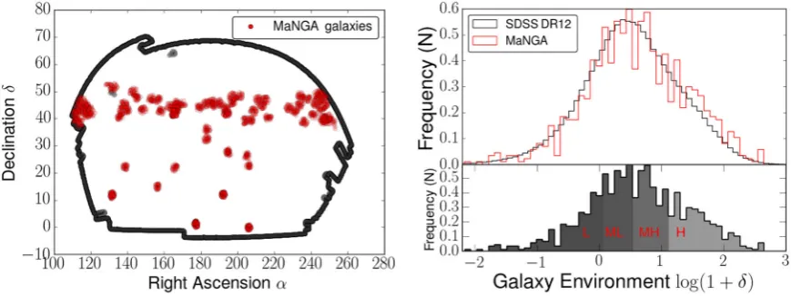
The MaNGA survey (Bundy et al.2015) is part of the fourth genera-tion of the SDSS and aims to obtain spatially resolved spectroscopy of nearly 10 000 galaxies (median redshift z ∼ 0.03) by 2020. MaNGA uses the five different types of IFU, with sizes that range from 19 fibres (12.5 arcsec diameter) to 127 fibres (32.5 arcsec diam-eter), to optimize these observations. Fibre bundle size and galaxy redshift are selected such that the fibre bundle provides the desired radial coverage [see Wake et al. (in preparation) for further details on sample selection and bundle size optimization and Law et al. (2015) for observing strategy]. In this work, we selected an original sample of 806 galaxies from the MaNGA data release MPL4 (equivalent to the public release SDSS DR13,www.sdss.org/dr13; SDSS Collab-oration2016), that were observed during the first year of operation (see Fig.1). The observational data were reduced using the MaNGA data-reduction-pipeline (Law et al.2016) and then analysed using the MaNGA data analysis pipeline (DAP; Westfall et al., in prepa-ration). To classify galaxies by morphology, we used Galaxy Zoo (Lintott et al.2011). In this work, we split the galaxies into two sub-sets, namely the ‘Early-type’ galaxies (Elliptical/Lenticular) and the ‘Late-type’ galaxies (Spiral/Irregular). Galaxies with an 80 per cent majority vote for a specific morphological type from the Galaxy Zoo were selected for this analysis. Galaxies that did not fulfil this criterion were visually inspected and classified by the authors.

2.2 Full spectral fitting

The spectral-fitting codeFIREFLY[see Wilkinson et al.2015,2016 for more details] and the models of Maraston & Str¨omb¨ack (2011) are used to derive stellar population properties from MaNGA DAP Voronoi binned spectra withS/N>5. This is different to the work of Zheng et al. (2016), where the full spectral fitting codeSTARLIGHT (Cid Fernandes et al.2005) and stellar population models of Bruzual & Charlot (2003), with a Chabrier (2003) initial mass function (IMF), are used. A full comparison on the choice of fitting codes and models can be found inPaper 1.

FIREFLY uses a χ2 _{minimization technique}1 _{that, given an} in-put spectral energy distribution (SED), returns a set of typically 100–1000 model fits. These initial fits are then checked to see

1_{Calculated asχ}2₌

λ(O(λ)−M(λ))

2

Figure 1. The left-hand plot shows a section of the SDSS footprint and the red circles highlight the positions of the observed MaNGA galaxies. The right-hand plot shows a comparison of galaxy environments derived for the SDSS DR12 subsample and for the MaNGA galaxy in this paper. For the DR12 sub-sample, we imposed a redshift cut ofz<0.15 (as this is the upper redshift limit of the MaNGA survey) and a magnitude cut in therband ofMr= −20. The red labels

L, ML, MH and H correspond to the different environmental density percentiles. whether their χ2 _{values can be improved by adding a different} simple stellar population component with luminosity equal to the first one. This process is then iterated until the χ2_{is minimized} and the solution cannot be improved by a statistically significant amount, which is governed by the Bayesian information criterion (Liddle2007). Prior to fitting the model templates to the data,FIREFLY takes into account galactic and interstellar reddening of the spectra. Foreground Milky Way reddening is accounted for by using the foreground dust maps of Schlegel, Finkbeiner & Davis (1998) and the extinction curve from Fitzpatrick (1999). The dust attenuation of each source is determined in the following way. The model tem-plates and data are pre-processed using a ‘High-Pass Filter (HPF)’. The HPF uses an analytic function across all wavelengths to rectify the continuum before deriving the stellar population parameters, allowing the removal of large-scale features (continuum shape and dust extinction).

FIREFLYrequires two additional inputs provided by the DAP; mea-surements of the stellar velocity dispersionσand fits to the strong nebular lines. Stellar velocity dispersion is needed to effectively remove the influence of the stellar kinematics on the stellar pop-ulation fit, and this is determined using the penalized pixel-fitting (pPXF) method of Cappellari & Emsellem (2004). The MaNGA DAP also fits individual Gaussians to the strong nebular emission lines after subtracting the best-fitting stellar-continuum model from the pPXF. The best-fitting parameters for all the fitted lines [OII], [OIII], [OI], Hα, Hβ, [NII] and [SII] are used to construct a model, emission-line only spectrum for each binned spectrum. These mod-els are subtracted from the binned spectra to produce emission-free spectra for analysis usingFIREFLY.

2.3 Radial gradients

The effective radiusRe, position angle and ellipticity of each galaxy are measured from SDSS photometry by performing a one compo-nent, two-dimensional Se´rsic fit in ther-band (Blanton et al.2005a). The on-sky position (relative to the galaxy centre) of each Voronoi cell is then used to calculate the semimajor axis coordinates, which we then use to define a radiusRof the cell. We define the radial gra-dient of a stellar population propertyθ(e.g. log (Age(Gyr)), [Z/H]) in units of dex/Reas:

∇θ=dθ/dR, (1)

whereRis the radius in units of effective radiusRe. The gradient is measured using least-squares linear regression (see Fig.2). Er-rors on the gradients are calculated using a Monte Carlo bootstrap resampling method (Press et al.2007).

2.4 Final sample

Due to the complex geometry of the SDSS footprint (which con-sists of an array of parabolic strips), some MaNGA galaxies that reside close to the footprint edge had to be excluded from the anal-ysis because an accurate measure of environment was not possible (see left-hand panel of Fig.1). Furthermore, a number of galaxies that were in the final morphologically classified sample had to be neglected from the final analysis due to having unreliable velocity dispersion estimates from the DAP. This led to the exclusion of 85 galaxies (33 early-type galaxies and 52 late-type galaxies span-ning a range of environments and masses) from our original sample of 806 galaxies, leaving 505 early-type galaxies and 216 late-type galaxies (70 per cent and 30 per cent of the sample, respectively).

3 G A L A X Y E N V I R O N M E N T

A galaxy’s environment is often expressed as the density field in which it resides. To quantify galaxy environment, a plethora of different indicators can be used. This can range from fixed aperture methods, which involve choosing a circle of radiusraround the galaxy in question and counting how many galaxies fall inside this circle giving a number density, to more complex methods taking into account redshift space distortions (Cooper et al.2005; Schawinski et al. 2007) and tidal tensor prescriptions based on the Hessian of the gravitational potential (Eardley et al.2015). These methods probe different environmental scales, so it is essential to choose the appropriate method that explores the desired range of the study.

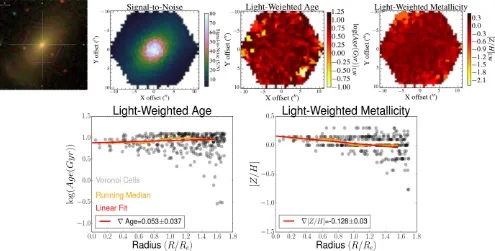
Figure 2. An example early-type galaxy from the MaNGA survey (MaNGA ID 1-114998) that has been observed with the 61 fibre IFU. The top row (from left to right) shows the SDSS image of the galaxy, the corresponding signal-to-noise map and the light-weighted age and metallicity maps derived fromFIREFLY, respectively. The bottom row shows the radial profiles of light-weighted age and metallicity for the galaxy, where the grey circles represent individual Voronoi cells from the DAP data cube, the orange line shows the running median and the red line shows the least-squares fit. The gradient value and corresponding error are quoted in the legend.

3.1 Local density

In this work, we look at local galaxy environment that is well determined usingNth nearest neighbour methods; see Muldrew et al. (2012) for a review. This method requires choosing a number Nof neighbours, calculating the distance to theNth neighbour and constructing a volume with this radius. DividingNby this volume gives the number density. Dense environments are obtained when theNth nearest neighbour is close to the target galaxy. The redshift range for neighbouring galaxies is±zc=1000 km s−1_{. We select}

N=5 and utilize an algorithm developed in Etherington & Thomas (2015). It was shown in Baldry et al. (2006) that the best estimate of local environment was an average ofN=4 and 5, hence we chose a value ofNclose to this to obtain robust measurements.

A local overdensityδis defined as:

δ= ρi−ρm

ρm

, (2)

whereρiis the number density described usingNth neighbour and

ρmis the mean density of galaxies within a redshift window centred on the target galaxy utilizing all the available area. A galaxies environment is then given by:

log(1+δ). (3)

From these measurements, we construct the distribution of envi-ronments for the MaNGA galaxy sample and compare this to the distribution of environments calculated for a magnitude and red-shift matched sample of SDSS DR12 galaxies (Alam et al.2015). This is to ensure that we were not biasing our measurements and only sampling MaNGA galaxies from particular environmental den-sities. The right-hand panel of Fig.1 shows this distribution of environments for the MaNGA galaxy sample compared to the en-vironments of the SDSS DR12 sample. This demonstrates that the

environmental densities of the MaNGA sample used here are rep-resentative of the environmental density distribution derived from a much larger, statistically complete sample.

We split the MaNGA environment distribution into quartiles to define four different environmental densities (see bottom-right panel of Fig.1). Galaxies were then assigned to one of these groups.

(i)δ <25th percentile=Lowδ;

(ii) 25th percentile< δ <50th percentile=Mid-Lowδ; (iii) 50th percentile< δ <75th percentile=Mid-Highδand (iv)δ >75th percentile=Highδ.

The number of galaxies in each environmental bin for our final analysis is 180, 178, 182 and 181, respectively. The distribution of galaxy masses that make up these bins can be seen in Fig.3. It can be seen that each bin of environmental density samples the full mass range and recovers well the mass–density relation, where the most massive galaxies live in the densest environments (Baldry et al.2006).

3.2 Mass-dependent environmental measure

Figure 3. Distributions of stellar mass [log (M/M)] for the four different environmental bins that make up the sample used in this work. Galaxy masses are drawn from the Nasa Sloan Atlas catalogue (NSA1). The mean

μand 1σvalue of each distribution are quoted in the panels.

a central galaxy with respect to its internal binding forces (Argudo-Fern´andez et al.2013,2014,2015). For one neighbour,Qipis given by:

Qip=

FTidal

FBinding

∝_MMi

p

_D

p

Rip

3

, (4)

whereMiis the mass of the neighbouring galaxy,Mpis the mass of the primary galaxy,Dpis the apparent diameter of the galaxy estimated by an isophote containing 90 per cent of the totalr-band flux of the galaxy and Rip is the projected distance between the neighbour and primary galaxy. Assuming a linear mass–luminosity relation (Bell et al.2003,2006), the stellar mass is proportional to ther-band flux at a fixed distance, withmr= −2.5 log (fluxr). The formula for one neighbour can be written as:

Qip=0.4

mp r−mir

+3 log

Dp

Rip

, (5)

wheremp

randmirare the apparent magnitudes in ther-band of the

primary galaxy and the neighbour, respectively. The tidal parameter Qforngalaxies is then defined as the dimensionless quantity of the gravitational interaction strength created by all the neighbours in the field:

Q=log _n

i=1

Qip . (6)

A low value ofQimplies that the primary galaxy is well isolated from external influences. The Spearman’s rank correlation coef-ficient between the environments calculated from theNth nearest neighbour method and theQparameter is 0.4 (see Fig.4).

3.3 Central and satellite galaxies

Most galaxies in the Universe are situated in many body systems. This can range from dense clusters of thousands of galaxies to galaxy pairs. The central galaxies in clusters tend to be the most luminous and most massive galaxies in the Universe and reside at the potential minimum of the dark matter halo. These galaxies also seem to be drawn from a different luminosity function compared to most other bright elliptical galaxies (Bernstein & Bhavsar2001),

Figure 4. Figure showing the comparison between the environments cal-culated using theNth nearest neighbour method and theQparameter. The red points represent individual galaxies used in this work, the grey contours represent the density of points. The Spearman’s rank correlation coefficient is 0.4.

thus hinting at a different evolutionary process. Satellite galaxies – galaxies moving relative to the potential minimum (having fallen into the larger halo) – are also thought to have unique evolutionary signatures. Their star formation is thought to be rapidly quenched when gas is removed due to ram pressure stripping. Therefore, it is interesting to consider how stellar population gradients in central and satellite galaxies change as a function of local environment. In order to separate the MaNGA galaxy sample used in this work into central/satellite galaxies, we use the halo-based group finder developed by Yang et al. (2007).

In Yang et al. (2007), all galaxies from the SDSS with z < 0.20 and anr-band magnitude brighter than 18 mag were selected and a halo-based group finder was used to identify the location of galaxies within different dark matter haloes. Once these haloes had been identified, the most luminous galaxies were defined as central galaxies and the others were defined as satellite galaxies. We then cross-matched the MaNGA galaxy sample used in this work to this catalogue. We classified 478 central galaxies and 243 satellite galaxies and use ourNth nearest neighbour measurements of environment to investigate whether stellar population gradients are different in central and satellite galaxies and whether there are possible dependences on local environmental density. The satellite fraction of∼33 per cent used in this work is an appropriate represen-tation of the local galaxy population, as it is similar to the fraction obtained in the larger MaNGA parent sample (∼31 per cent) and to the fraction calculated atz∼0.03 in the complete Yang et al. (2007) catalogue (∼30 per cent).

4 R E S U LT S

In Paper 1, we find that early-type galaxies generally ex-hibit shallow light-weighted age gradients [∇log (Age(Gyr))LW∼

−0.004 dex/Re] and slightly positive mass-weighted age gra-dients [∇log (Age(Gyr))MW ∼ 0.092 dex/Re]. Light- and mass-weighted metallicity gradients tend to be negative (∇[Z/H]LW

∇[Z/H]LW ∼ −0.13 dex−1), Spolaor et al. (2009) (∇[Z/H]LW ∼

−0.16 dex/Re), and modern cosmological simulations (Hirschmann et al. 2015). However, our light-weighted metallicity gradients are shallower than what is found by Kuntschner et al. (2010) (∇[Z/H]LW= −0.28±0.12 dex/Re). There are a number of possible reasons for this difference in gradient value. First, the choice of stel-lar population models and stelstel-lar library is important when deriving gradients. It was shown inPaper 1[and can be seen in Gonz´alez Delgado et al. (2015)], that the use of different models can lead to offsets in the derived gradients by 0.1−0.3 dex. Secondly, de-pending on the spatial resolution of the data, beam smearing can flatten out the inferred radial gradient. SAURON data are used in Kuntschner et al. (2010), which have much higher spatial resolu-tion than the MaNGA data. However, the effect of beam smearing was investigated inPaper 1and we found no significant impact on our gradients. Lastly, the radial range over which the gradient is calculated can also have a significant effect on the gradient, as it was shown in Gonz´alez Delgado et al. (2015), that different gra-dients can be found in the inner and outer regions of a galaxy. A comprehensive discussion of the derived metallicity gradients from the literature is provided inPaper 1, and the median literature on metallicity gradient was found to beμ= −0.20, with a spreadσ= 0.11. Our result, and that of Kuntschner et al. (2010), sits reasonably well within this range.

For late-type galaxies, we find negative light-weighted age gradi-ents [∇log (Age(Gyr))LW∼ −0.11 dex/Re] and flat mass-weighted age gradients (∇log (Age(Gyr))MW ∼0.01 dex/Re). Both light-and mass-weighted metallicity gradients are found to be negative (∇[Z/H]LW∼ −0.07 dex/Re,∇[Z/H]MW ∼ −0.10 dex/Re), simi-lar to what was found in the CALIFA survey (S´anchez-Bl´azquez et al.2014; Gonz´alez Delgado et al.2015) and consistent with the inside-out formation of disc galaxies.

InPaper 1, we also investigated the relationship between stellar population gradients and stellar mass by fitting linear relationships in the gradient–mass plane. We found that no correlation exists be-tween age gradients and mass for both early- and late-type galaxies. However, there is a correlation between the negative metallicity gra-dients and mass, where the gragra-dients become steeper with increasing galaxy mass, agreeing with what was found in Gonz´alez Delgado et al. (2015). In this section, we break these results down further and investigate the relationship between the stellar population gradients of both early- and late-type galaxies with galaxy environment, as described by three independent environment measures.

4.1 Local density

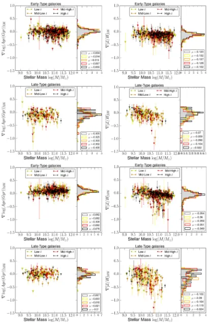
Fig.5shows the derived light- and mass-weighted stellar popu-lation gradients as a function of stellar mass log (M/M) for the four different environmental densities defined using theNth nearest neighbour method. Additionally, Table 1shows the correspond-ing median gradients with 1σ errors for each environment. For early-type galaxies, the light- and mass-weighted stellar population gradients appear to be fairly homogenous across the different en-vironments and are in good agreement with the gradients obtained for the whole sample. Light- and mass-weighted ages, for each en-vironmental density, fluctuate around∼0 dex/Reand∼0.9 dex/Re, and light- and mass-weighted metallicities tend to be negative, with values around∼−0.12 dex/Re and ∼−0.05 dex/Re, respectively. The story is similar for late-types, where light- and mass-weighted ages are fairly consistent across the different environments, yielding median gradient values of∼−0.1 dex/Reand∼0 dex/Re.

Metallic-ity gradients tend to have a greater scatter, but there is no significant deviation from one environmental density to another.

To further test our conclusions, we conducted simple Kolmogorov–Smirnov (K–S) tests on the distributions of gradients for the different environmental densities. The K–S test allows us to check whether two distributions are drawn from the same underly-ing distribution. If environmental effects are notable, there will be a significant difference when comparing the cumulative distribution functions of the two most contrasting environmental densities. For this reason, we conducted our K–S tests on the low-δand high-δ distributions.2_{Results of this analysis can be seen in Table2.}

Overall we see that for both early- and late-type galaxies, the cumulative distributions of gradients do not differ much between the lowest and highest density environments, withp-values rang-ing between 0.25 and 0.91. For light-weighted metallicity gradients in early-type galaxies however, there seems to be some difference between the two distributions withp-value= 0.01±0.10. Thus suggesting being drawn from different underlying distributions and evidence for some environmental dependence. The error, obtained via Monte Carlo bootstrap resampling, on this value is quite large, and therefore we cannot conclusively say that there is an environ-mental dependence on the light-weighted metallicity gradients of early-types.

As mentioned previously, inPaper 1we look at relationships between stellar population gradients and stellar mass by fitting lin-ear relationships in the gradient–mass plane. We can extend this exercise here by fitting these relations to each of the different en-vironmental densities to see if there is any enen-vironmental effect on this mass dependence. Table3shows the slopes of the relationship between stellar population gradient and galaxy mass for the various environmental density bins and galaxy types. There appears to be no significant slope for both early- and late-type galaxies, suggesting that there is no dependence of these relationships on environmental density.

4.2 Mass-dependent environmental measure

Our analysis using the tidal strength estimator followed in exactly the same vein as before and galaxies were classified into four dif-ferent environmental densities (lowQ, mid-lowQ, mid-highQand highQ). The results of this analysis is shown in Fig.6, where we plot the stellar population gradient as a function of different environmen-tal densities. Overall, we find that the light-weighted age gradients for both early- and late-type galaxies do not vary between different environments, with values of∼0 dex/Reand∼−0.1 dex/Rebeing recovered. This is true also for the mass-weighted gradients, where gradient values in each density bin are∼0.1 dex/Reand∼0 dex/Re. Light- and mass-weighted metallicity gradients for both early- and late-type galaxies also show no significant dependence on the envi-ronment, with median values of∼−0.15 dex/Re,∼−0.05 dex/Re,

∼−0.05 dex/Reand∼−0.1 dex/Rebeing recovered in the different density bins.

To conclude, we find no dependence of stellar population gradi-ents on this alternative measurement of environmental density. This further strengthens the conclusion that we presented in the section

2_{In an attempt to account for the errors on the individual gradients when}

Table 1. Median light and mass-weighted gradients for both early- and late-type galaxies. The gradients are split by different environmental densities. Errors correspond to the 1σvalue from the distribution.

Morphology Property Lowδ Mid-lowδ Mid-highδ Highδ

∇(dex/Re) ∇(dex/Re) ∇(dex/Re) ∇(dex/Re)

Early-type Mass-weighted Age 0.092±0.10 0.108± 0.08 0.092±0.08 0.078±0.07 Light-weighted Age −0.014±0.09 0.013± 0.08 −0.007±0.09 −0.009±0.07 Mass-weighted [Z/H] −0.06±0.09 −0.059± 0.08 −0.051±0.09 −0.049±0.07 Light-weighted [Z/H] −0.132±0.09 −0.137± 0.08 −0.128±0.07 −0.102±0.07 Late-type Mass-weighted Age 0.03±0.12 0.016± 0.15 0.021±0.16 −0.01±0.20 Light-weighted Age −0.125±0.12 −0.109± 0.15 −0.102±0.17 −0.106±0.20 Mass-weighted [Z/H] −0.09±0.12 −0.164± 0.15 −0.119±0.16 −0.024±0.20 Light-weighted [Z/H] −0.059±0.12 −0.096± 0.14 −0.104±0.15 −0.02±0.19

Table 2. Table showing the corresponding Kolmogorov–Smirnov statistic (K–S) andp-value (P) for the empirical cumulative distribution function (ECDF) of the lowest and highest environmental densities. As the K–S test only cares about the raw gradient value, errors on the K–S statistic and p-values were calculated via Monte Carlo methods to attempt to account for the errors on the individual gradients.

Morphology Property K–S Statistic p-value Early-types Light-weighted Age 0.01±0.04 0.55±0.24

Mass-weighted Age 0.12±0.04 0.37±0.16 Light-weighted [Z/H] 0.21±0.07 0.01±0.10 Mass-weighted [Z/H] 0.11±0.04 0.48±0.20 Late-types Light-weighted Age 0.10±0.06 0.91±0.25 Mass-weighted Age 0.24±0.09 0.25±0.25 Light-weighted [Z/H] 0.15±0.06 0.78±0.27 Mass-weighted [Z/H] 0.16±0.07 0.69±0.27

above using theNth nearest neighbour method, that the gradients of both early- and late-type galaxies are at most weakly dependent on environment.

4.3 Central and satellite galaxies

Fig.7shows the light-weighted age and metallicity gradients for central (grey) and satellite (red) galaxies, as a function of local environment. Table4shows the numerical results of this analysis. First, Fig.7shows that stellar population gradients are indepen-dent of environmental density, as no correlation is eviindepen-dent between stellar population gradient and local density. This can be quan-titively described by fitting a line through the stellar population gradient–environment plane in each panel plot. We find that lumi-nosity and mass-weighted stellar population gradients generally do not correlate with local environment neither for central nor satellite galaxies. We further do not detect any evidence for a difference in gradients between satellite and central galaxies (see also Table4). We conclude that the galaxy environment, whether measured as lo-cal environmental density or through central/satellite classification, does not appear to have any significant effect on age and metallic-ity gradients in galaxies. This result agrees well with a recent IFU study of nearby massive galaxies as part of the MASSIVE survey, where it is found that even at large radius, internal properties mat-ter more than environment in demat-termining star formation history (Greene et al.2015).

4.4 Environmental trends

To ensure that our galaxy sample size was sufficient to identify different environmental impacts on gradients, we attempted to

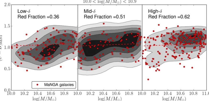
reproduce known environmental trends on galaxy properties. Peng et al. (2010) studied the fraction of red galaxies as a function of environment and mass and found higher fractions of red galaxies exist in denser environments. We took a sample of galaxies in our study (10< log (M/M) < 10.9), and calculated the red frac-tion for three different environment bins. The bins were defined in a similar fashion to what was done for theNth nearest neigh-bour, using percentiles of the environment distribution. First, the (u−g)RESTcolour for each galaxy was calculated using:

(u−g)REST=(u−g)−kug (7)

wherekugis theK-correction that is small for the low-redshift galaxy sample used in this work (kug≈0.05 mag). Secondly, we used the transform equation of Lupton (2005), found on the SDSS website, to get (U−B)RESTcolours

(U−B)REST=0.8116((u−g)REST)−0.1313. (8) Lastly, following the prescription of Peng et al. (2010), a dividing line was then employed so that we could define different galaxy populations. The dividing line has the form:

(U−B)REST=1.10+0.075 log(m/1010M)−0.182. (9) Galaxies with (U−B)REST greater than this were classed as red, and galaxies under this line were classed as blue (see Fig. 8). We find that in the lowest density environments, the red frac-tion is 36 per cent and then increases up to 50 per cent in the next environmental density. In the highest density environment, the fraction of red galaxies increases to 60 per cent. This trend is similar to that found in Peng et al. (2010). It is reassuring that environmental effects can be detected with the present density es-timates and sample size. Hence, any significant trends between stellar population gradient and environment are detectable with the present sample, and if there are any residual dependences of stellar population gradients on environment, they must be a very subtle.

5 D I S C U S S I O N

Late-type galaxies

Figure 6. Figure showing the median gradients obtained in different environmental densities using theQparameter. Top panels show early-type galaxies and bottom panels show late-type galaxies. From left to right, the plots show the light-weighted age, mass-weighted age, light-weighted [Z/H] and mass-weighted [Z/H]. The error bars correspond to the standard deviation of the distribution.

feedback, matter most in determining the stellar population gradi-ents in galaxies. Fig.6, which shows the stellar population gradients as a function of environment using the mass-dependant parameter Q, also corroborates with this view, as the gradients are relatively homogeneous across theQspectrum.

In the parallel paper of Zheng et al. (2016), the same lack of envi-ronmental dependence was found, agreeing with what is presented here. They find that disc galaxies have negative age and metallicity gradients, and elliptical galaxies have flat age gradients and nega-tive metallicity gradients, qualitanega-tively agreeing with our gradient values. These gradient values also remain consistent between the cluster, filament, sheet and void classification, showing no impact of environment. It is reassuring to see that a study using differ-ent methods, such as environmdiffer-ent classification, full spectral-fitting code and stellar population models, can produce similar conclusions to what is presented in this study.

Another way of investigating environmental effects on stellar population gradients is to look at the difference between central and

satellite galaxies, as these will be exposed to numerous different physical processes that can influence their evolution. Fig.7shows the gradients obtained for central and satellite galaxies as a function ofNth nearest neighbour environmental density. We find that both central and satellite galaxies have relatively flat age gradients and negative metallicity gradients. This highlights the importance of internal properties, as opposed to location in the dark matter halo, on the inferred radial gradients. Table4shows the gradient values for the central and satellite galaxies as a function of four different environmental densities, and once again, no significant trend of the gradients of central and satellite galaxies with local environment is present. A study by Brough et al. (2007) found similar results when investigating a sample of brightest group galaxies and brightest cluster galaxies.

Figure 7. Light- (top) and mass-weighted (bottom) stellar population gradients in age and metallicity for central (grey) and satellite (red) galaxies as a function of environmental density. Central galaxies that have no satellite companions in their dark matter halo are shown by circular markers. The distributions in the top panels shows the distribution of environments for the central and satellite galaxies, the right-hand panels show the distributions of the gradients for centrals and satellites, respectively.

Table 4. Median light- and mass-weighted age/metallicity gradients obtained for the 478 central and 243 satellite galaxies from the MaNGA galaxy sample, for different environmental densities. Errors on the quantities are given by 1/√NwhereNis the number of galaxies in that specific bin.

Property Classification Lowδ Mid-lowδ Mid-highδ Highδ

∇(dex/Re) ∇(dex/Re) ∇(dex/Re) ∇(dex/Re)

Light-weighted Age Central −0.01±0.05 −0.04±0.06 −0.03± 0.06, −0.01±0.05 Satellite 0.01±0.07 −0.02±0.08 0.01± 0.06 −0.01±0.07 Mass-weighted Age Central 0.06±0.05 0.11±0.06 0.10± 0.06 0.08±0.05 Satellite 0.10±0.07 0.12±0.08 0.09± 0.06 0.08±0.07 Light-weighted [Z/H] Central −0.14±0.05 −0.10±0.06 −0.10± 0.06 −0.11±0.05 Satellite −0.15±0.07 −0.11±0.08 −0.13± 0.06 −0.11±0.07 Mass-weighted [Z/H] Central −0.03±0.05 −0.07±0.06 −0.01± 0.06 −0.05±0.05 Satellite −0.09±0.07 0.04±0.08 −0.05± 0.06 0.04±0.07

galaxies from SDSS imaging. They find that in most cases, age and metallicity gradients generally do not depend on environmental density. However, a mild residual dependence of metallicity gradient with environment is seen for central galaxies only, a pattern not detected here. This mild residual dependence has also been found in studies by S´anchez-Bl´azquez, Gorgas & Cardiel (2006b), using 82 galaxies in the coma cluster, and La Barbera et al. (2011b) who used optical and near-infrared colours to study group and field galaxies. It will be interesting in future to see whether such

a residual dependence can be recovered with larger MaNGA galaxy samples or alternative methodologies in future studies.

6 C O N C L U S I O N S

Figure 8. Figure showing the colour–mass relation for three different environmental densities. The grey contours represent the density of points, the red circles show the MaNGA galaxies and the red dividing line distinguishes the red and blue galaxies from Peng et al. (2010). The red fraction of galaxies is shown in each corresponding panel. All galaxies have a mass in the range 10<log (M/M)<10.9.

age and metallicity within 1.5Re, for a representative sample of 721 galaxies taken from the first year of MaNGA observations (MPL4, equivalent to DR13) with masses ranging from 109_{to 10}11.5_M

. We split our galaxy sample into 505 early- and 216 late-type galaxies based on Galaxy Zoo classifications and analyse the impact of galaxy environment on the stellar population gradients. We calcu-late local environmental densities from the SDSS parent catalogue using Nth nearest neighbour. In addition to this, we also look at a mass-dependent environmental measure,Q, which quantifies the tidal strength of nearest neighbours and split the MaNGA sample into central and satellite galaxies.

We then apply the full spectral-fitting codeFIREFLYon these spec-tra to derive the stellar population parameters averaged age and metallicity. We use the stellar population models of Maraston & Str¨omb¨ack (2011) (M11), which utilize the MILES stellar library (S´anchez-Bl´azquez et al.2006a) and assume a Kroupa stellar IMF (Kroupa 2001). In our analysis, we find that early-type galaxies generally exhibit shallow light-weighted age gradients in agree-ment with the literature. However, the mass-weighted median age does show some radial dependence with positive gradients. Late-type galaxies, instead, have negative light-weighted age gradients in agreement with the literature. We generally detect negative metal-licity gradients for both early- and late-types at all masses, but these are significantly steeper in late-type compared to early-type galaxies.

To understand the impact of galaxy environment on stellar pop-ulation gradients, the galaxy sample was further split into four different local environmental densities. Distributions of age and metallicity gradients turn out to be indistinguishable across the different environments, and we also do not find any correlation be-tween stellar population gradient and local density. The K–S tests were conducted to confirm this result for both early- and late-type galaxies. In addition to this, we repeated our analysis using the tidal strength parameterQ. This mass-dependent environment measure yielded similar results and the gradients appear to be indistinguish-able across the different environments. We also split the sample into central and satellite galaxies and found that both the

light-and mass-weighted age light-and metallicity gradients are the same for both classes, and their values also do not vary across different en-vironments. We therefore conclude that galaxy environment has no significant effect on age or metallicity gradients in galaxies at least within 1.5Re, independently of mass or type. Hydrodynamical simulations of galaxy formation from the literature predict age gra-dients in early-type galaxies to be generally flat and independent of galaxy mass or environment, which agrees well with the findings of this paper. However, galaxy formation simulations seem to predict a dependence of metallicity gradients on environment, which is not confirmed by the results of the present study. A more comprehensive and direct comparison between MaNGA observations and predic-tions from galaxy formation simulapredic-tions will be very valuable in future.

AC K N OW L E D G E M E N T S

Institute for the Physics and Mathematics of the Universe (IPMU) / University of Tokyo, Lawrence Berkeley National Laboratory, Leibniz Institut fr Astrophysik Potsdam (AIP), Max-Planck-Institut fr Astronomie (MPIA Heidelberg), Max-Planck-Institut fr Astro-physik (MPA Garching), Max-Planck-Institut fr Extraterrestrische Physik (MPE), National Astronomical Observatory of China, New Mexico State University, New York University, University of Notre Dame, Observatrio Nacional/MCTI, The Ohio State University, Pennsylvania State University, Shanghai Astronomical Observa-tory, United Kingdom Participation Group, Universidad Nacional Autnoma de M´exico, University of Arizona, University of Colorado Boulder, University of Oxford, University of Portsmouth, Univer-sity of Utah, UniverUniver-sity of Virginia, UniverUniver-sity of Washington, Uni-versity of Wisconsin, Vanderbilt UniUni-versity, and Yale UniUni-versity.

All data taken as part of SDSS-IV is scheduled to be released to the community in fully reduced form at regular intervals through dedicated data releases. The first MaNGA data release was part of the SDSS data release 13 (release date – 2016 July 31).

R E F E R E N C E S

Alam S. et al., 2015, ApJS, 219, 12 Allen J. T. et al., 2015, MNRAS, 446, 1567 Argudo-Fern´andez M. et al., 2013, A&A, 560, A9 Argudo-Fern´andez M. et al., 2014, A&A, 564, A94 Argudo-Fern´andez M. et al., 2015, A&A, 578, A110 Bacon R. et al., 1995, A&AS, 113, 347

Baldry I. K., Balogh M. L., Bower R. G., Glazebrook K., Nichol R. C., Bamford S. P., Budavari T., 2006, MNRAS, 373, 469

Bell E. F., McIntosh D. H., Katz N., Weinberg M. D., 2003, ApJS, 149, 289 Bell E. F., Phleps S., Somerville R. S., Wolf C., Borch A., Meisenheimer

K., 2006, ApJ, 652, 270

Bernstein J. P., Bhavsar S. P., 2001, MNRAS, 322, 625

Bershady M. A., Verheijen M. A. W., Swaters R. A., Andersen D. R., Westfall K. B., Martinsson T., 2010, ApJ, 716, 198

Bershady M. A., Martinsson T. P. K., Verheijen M. A. W., Westfall K. B., Andersen D. R., Swaters R. A., 2011, ApJ, 739, L47

Blanton M. R., Moustakas J., 2009, ARA&A, 47, 159 Blanton M. R. et al., 2005a, AJ, 129, 2562

Blanton M. R., Eisenstein D., Hogg D. W., Schlegel D. J., Brinkmann J., 2005b, ApJ, 629, 143

Brough S., Proctor R., Forbes D. A., Couch W. J., Collins C. A., Burke D. J., Mann R. G., 2007, MNRAS, 378, 1507

Bruzual G., Charlot S., 2003, MNRAS, 344, 1000 Bundy K. et al., 2015, ApJ, 798, 7

Cappellari M., Emsellem E., 2004, PASP, 116, 138 Cappellari M. et al., 2011, MNRAS, 413, 813 Chabrier G., 2003, PASP, 115, 763

Cid Fernandes R., Mateus A., Sodr´e L., Stasi´nska G., Gomes J. M., 2005, MNRAS, 358, 363

Colless M. et al., 2001, MNRAS, 328, 1039

Cooper M. C., Newman J. A., Madgwick D. S., Gerke B. F., Yan R., Davis M., 2005, ApJ, 634, 833

Davies R. I., M¨uller S´anchez F., Genzel R., Tacconi L. J., Hicks E. K. S., Friedrich S., Sternberg A., 2007, ApJ, 671, 1388

Davis M., Efstathiou G., Frenk C. S., White S. D. M., 1985, ApJ, 292, 371 de Zeeuw P. T. et al., 2002, MNRAS, 329, 513

Dressler A., 1980, ApJ, 236, 351

Eardley E. et al., 2015, MNRAS, 448, 3665 Etherington J., Thomas D., 2015, MNRAS, 451, 660 Farouki R., Shapiro S. L., 1981, ApJ, 243, 32 Fitzpatrick E. L., 1999, PASP, 111, 63

Goddard D. et al., 2016, MNRAS, in press (Paper I) Gonz´alez Delgado R. M. et al., 2015, A&A, 581, A103

Greene J. E., Janish R., Ma C.-P., McConnell N. J., Blakeslee J. P., Thomas J., Murphy J. D., 2015, ApJ, 807, 11

Guth A. H., 1981, Phys. Rev. D, 23, 347

Hahn O., Carollo C. M., Porciani C., Dekel A., 2007, MNRAS, 381, 41 Hirschmann M., Naab T., Ostriker J. P., Forbes D. A., Duc P.-A., Dav´e R.,

Oser L., Karabal E., 2015, MNRAS, 449, 528 Hogg D. W. et al., 2004, ApJ, 601, L29 Kamann S. et al., 2016, The Messenger, 164, 18

Kauffmann G., White S. D. M., Heckman T. M., M´enard B., Brinchmann J., Charlot S., Tremonti C., Brinkmann J., 2004, MNRAS, 353, 713 Kroupa P., 2001, MNRAS, 322, 231

Kuntschner H. et al., 2010, MNRAS, 408, 97

La Barbera F., Ferreras I., de Carvalho R. R., Lopes P. A. A., Pasquali A., de la Rosa I. G., De Lucia G., 2011a, ApJ, 740, L41

La Barbera F., Ferreras I., de Carvalho R. R., Lopes P. A. A., Pasquali A., de la Rosa I. G., De Lucia G., 2011b, ApJ, 740, L41

Larson R. B., Tinsley B. M., Caldwell C. N., 1980, ApJ, 237, 692 Law D. R. et al., 2015, AJ, 150, 19

Law D. et al., 2016, AJ, 152, 83 Liddle A. R., 2007, MNRAS, 377, L74 Lintott C. et al., 2011, MNRAS, 410, 166

Maraston C., Str¨omb¨ack G., 2011, MNRAS, 418, 2785

McDermid R. M., Bacon R., Kuntschner H., 2006, New Astron. Rev., 49, 521

Mehlert D., Thomas D., Saglia R. P., Bender R., Wegner G., 2003, A&A, 407, 423

Mercurio A. et al., 2006, MNRAS, 368, 109 Muldrew S. I. et al., 2012, MNRAS, 419, 2670 Oemler A., Jr, 1974, ApJ, 194, 1

Peng Y.-j. et al., 2010, ApJ, 721, 193 P´erez E. et al., 2013, ApJ, 764, L1

Planck Collaboration XIII, 2016, A&A, 594, A13

Press W. H., Teukolsky S. A., Vetterling W. T., Flannery B. P., 2007, Nu-merical Recipes: The Art of Scientific Computing, 3rd edn. Cambridge Univ. Press, New York, NY

Rawle T. D., Smith R. J., Lucey J. R., 2010, MNRAS, 401, 852

Read J. I., Wilkinson M. I., Evans N. W., Gilmore G., Kleyna J. T., 2006, MNRAS, 366, 429

Riffel R. A., Storchi-Bergmann T., Riffel R., Pastoriza M. G., 2010, ApJ, 713, 469

Riffel R., Riffel R. A., Ferrari F., Storchi-Bergmann T., 2011, MNRAS, 416, 493

S´anchez S. F. et al., 2012, A&A, 538, A8

S´anchez-Bl´azquez P. et al., 2006a, MNRAS, 371, 703

S´anchez-Bl´azquez P., Gorgas J., Cardiel N., 2006b, A&A, 457, 823 S´anchez-Bl´azquez P. et al., 2014, A&A, 570, A6

Schawinski K. et al., 2007, ApJS, 173, 512

Schlegel D. J., Finkbeiner D. P., Davis M., 1998, ApJ, 500, 525 SDSS Collaboration, 2016, ApJS, preprint (arXiv:1608.02013)

Spolaor M., Proctor R. N., Forbes D. A., Couch W. J., 2009, ApJ, 691, L138 Storchi-Bergmann T., Riffel R. A., Riffel R., Diniz M. R., Borges Vale T.,

McGregor P. J., 2012, ApJ, 755, 87

Thomas D., Maraston C., Schawinski K., Sarzi M., Silk J., 2010, MNRAS, 404, 1775

Tortora C., Napolitano N. R., 2012, MNRAS, 421, 2478

Wang H., Mo H. J., Jing Y. P., Guo Y., van den Bosch F. C., Yang X., 2009, MNRAS, 394, 398

Wang H., Mo H. J., Yang X., van den Bosch F. C., 2012, MNRAS, 420, 1809

White S. D. M., Rees M. J., 1978, MNRAS, 183, 341 Wilkinson D. M. et al., 2015, MNRAS, 449, 328 Wilkinson D. M. et al., 2016, MNRAS, in press

Yang X., Mo H. J., van den Bosch F. C., Pasquali A., Li C., Barden M., 2007, ApJ, 671, 153

York D. G. et al., 2000, AJ, 120, 1579 Zheng Z. et al., 2016, ApJ, in press

1_{Institute of Cosmology and Gravitation, University of Portsmouth, Burnaby}

MD 21218, USA

10_{Department of Physics and Astronomy, University of Kentucky, 505 Rose}

St., Lexington, KY 40506-0057, USA

11_{Department of Physical Sciences, The Open University, Milton Keynes,}

UK

601, Antofagasta 1270300, Chile

21_{Departamento de F´ısica, Facultad de Ciencias, Universidad de La Serena,}

Cisternas 1200, La Serena, Chile