Stochastic Attribute Value Grammars

(1)

Stochastic Attribute-Value Grammars

S t e v e n P. A b n e y * AT&T Laboratories

Probabilistic analogues of regular and context-free grammars are well known in computational

linguistics, and currently the subject of intensive research. To date, however, no satisfactory

probabilistic analogue of attribute-value grammars has been proposed: previous attempts have

failed to define an adequate parameter-estimation algorithm.

In the present paper, I define stochastic attribute-value grammars and give an algorithm

for computing the maximum-likelihood estimate of their parameters. The estimation algorithm

is adapted from Della Pietra, Della Pietra, and Lafferty (1995). To estimate model parameters, it

is necessary to compute the expectations of certain functions under random fields. In the appli-

cation discussed by Della Pietra, Della Pietra, and Lafferty (representing English orthographic

constraints), Gibbs sampling can be used to estimate the needed expectations. The fact that

attribute-value grammars generate constrained languages makes Gibbs sampling inapplicable,

but I show that sampling can be done using the more general Metropolis-Hastings algorithm.

1. Introduction

Stochastic versions of regular grammars and context-free grammars have received a great deal of attention in computational linguistics for the last several years, and ba- sic techniques of stochastic parsing and parameter estimation have been known for decades. However, regular and context-free grammars are widely deemed linguisti- cally inadequate; standard grammars in computational linguistics are attribute-value (AV) grammars of some variety. Before the advent of statistical methods, regular and context-free grammars were considered too inexpressive for serious consideration, and even now the reliance on stochastic versions of the less-expressive grammars is often seen as an expedient necessitated by the lack of an adequate stochastic version of attribute-value grammars.

Proposals have been made for extending stochastic models developed for the regular and context-free cases to grammars with constraints. 1 Brew (1995) sketches a probabilistic version of Head-Driven Phrase Structure Grammar (HPSG). He proposes a stochastic process for generating attribute-value structures, that is, directed acyclic graphs (dags). A dag is generated starting from a single node labeled with the (unique) most general type. Each type S has a set of maximal subtypes T1 . . .

Tin.

To expand a node labeled S, one chooses a maximal subtype T stochastically. One then considers equating the current node with other nodes of type T, making a stochastic y e s / n o de-

* AT&T Laboratories, Rm. A249, 180 Park Avenue, Florham Park, NJ 07932

(2)

Computational Linguistics Volume 23, Number 4

cision for each. Equating two nodes creates a re-entrancy. If the current node is equated with no other node, one proceeds to expand it. Each maximal type introduces types U1 . . . Un, corresponding to values of attributes; one creates a child node for each introduced type, and then expands each child in turn. A limitation of this approach is that it permits one to specify only the average rate of re-entrancies; it does not permit one to specify more complex context dependencies.

Eisele (1994) takes a logic-programmhlg approach to constraint grammars. He assigns probabilities to proof trees by attaching parameters to logic program clauses. He presents the following logic program as an example:

1. p(X,Y,Z) +-1 q(X,Y), r(Y,Z).

2. q(a,b) +-0.4

3. q(X,c) +-0.6

4. r(b,d) +-0.5

5. r(X,e) +-o.5

The probability of a proof tree is defined to be proportional to the product of the probabilities of clauses used in the proof. Normalization is necessary because some derivations lead to invalid proof trees. For example, the derivation

p(x,Y,Z) Y~

q(X,Y) r(Y,Z) by3 r ( c , Z ) : Y=c

~y4

: Y=c b=c Z=d

is invalid because of the illegal assignment b = c.

Both Brew and Eisele associate weights with analogues of rewrite rules. In Brew's case, we can view type expansion as a stochastic choice from a finite set of rules of form X --* ~i, where X is the type to expand and each ~i is a sequence of introduced child types. A re-entrancy decision is a stochastic choice between two rules, X --* y e s and X --* no, where X is the type of the node being considered for re-entrancy. In Eisele's case, expanding a goal term can be viewed as a stochastic choice among a finite set of rules X ---* ~i, where X is the predicate of the goal term and each ~i is a program clause whose head has predicate X. The parameters of the models are essentially weights on such rules, representing the probability of choosing

~i

when making a choice of type X.

In these terms, Brew and Eisele propose estimating parameters as the empirical relative frequency of the corresponding rules. That is, the weight of the rule X ---+ ~i is obtained by counting the number of times X rewrites as ~i in the training corpus, divided by the total number of times X is rewritten in the training corpus. For want of a standard term, let us call these estimates Empirical Relative Fre- quency (ERF) estimates. To deal with incomplete data, both Brew and Eisele appeal to the Expectation-Maximization (EM) algorithm, applied however to ERF rather than maximum-likelihood estimates.

Under certain independence conditions, ERF estimates are maximum-likelihood estimates. Unfortunately, these conditions are violated when there are context dependencies of the sort found in attribute-value grammars, as will be shown below. As a consequence, applying the ERF method to attribute-value grammars' does n o t generally yield maximum-likelihood estimates. This is true whether one uses EM or n o t - - a method that yields the "wrong" estimates on complete data does not improve when EM is used to extend the method to incomplete data.

(3)

Abney Stochastic Attribute-Value Grammars

with the frequency of proof trees in the training corpus. Eisele recognizes that this problem arises only where there are context dependencies.

Fortunately, solutions to the context-dependency problem have been described (and indeed are currently enjoying a surge of interest) in statistics, machine learning, and statistical pattern recognition, particularly image processing. The models of interest are known as random fields. Random fields can be seen as a generalization of Markov chains and stochastic branching processes. Markov chains are stochastic processes corresponding to regular grammars and random branching processes are stochastic processes corresponding to context-free grammars. The evolution of a Markov chain describes a line, in which each stochastic choice depends only on the state at the immediately preceding time-point. The evolution of a random branching process describes a tree in which a finite-state process may spawn multiple child processes at the next time-step, but the number of processes and their states depend only on the state of the unique parent process at the preceding time-step. In particular, stochastic choices are

independent

of other choices at the same time-step: each process evolves independently. If we permit re-entrancies, that is, if we permit processes to re-merge, we generally introduce context-sensitivity. In order to re-merge, processes must be "in synch," which is to say, they cannot evolve in complete independence of one another. Random fields are a particular class of multidimensional random processes, that is, processes corresponding to probability distributions over an arbitrary graph. The theory of random fields can be traced back to Gibbs (1902); indeed, the probability distributions involved are known as Gibbs distributions.

To m y knowledge, the first application of random fields to natural language was Mark et al. (1992). The problem of interest was how to combine a stochastic context- free grammar with n-gram language models. In the resulting structures, the probability of choosing a particular word is constrained simultaneously by the syntactic tree in which it appears and the choices of words at the n preceding positions. The context- sensitive constraints introduced by the n-gram model are reflected in re-entrancies in the structure of statistical dependencies, as in Figure 1.

S

/ N

NP VP there was NP

k ~ J ~jno~sponse

Figure 1

Statistical dependencies under the model of Mark et al. (1992).

In this diagram, the choice of label on a node z with parent x and preceding word y is dependent on the label of x and y, but conditionally independent of the label on any other node.

Della Pietra, Della Pietra, and Lafferty (1995, henceforth, DD&L) also apply random fields to natural language processing. The application they consider is the induction of English orthographic constraints--inducing a grammar of possible English words. DD&L describe an algorithm called Improved Iterative Scaling (IIS) for selecting informative features of words to construct a random field, and for setting the parameters of the field optimally for a given set of features, to model an empirical word distribution.

(4)

grammars with probabilities. In brief, the difficulty is that the IIS algorithm requires the computation of the expectations, under random fields, of certain functions; in general, computing these expectations involves summing over all configurations (all possible character sequences, in the orthography application), which is not possible when the configuration space is large. Instead, DD&L use Gibbs sampling to estimate the needed expectations.

Gibbs sampling is possible for the application that DD&L consider. A prerequisite for Gibbs sampling is that the configuration space be closed under relabeling of graph nodes. In the orthography application, the configuration space is the set of possible English words, represented as finite linear graphs labeled with ASCII characters. Every w a y of changing a label, that is, every substitution of one ASCII character for a different one, yields a possible English word.

By contrast, the set of graphs admitted b y an attribute-value grammar G is highly constrained. If one changes an arbitrary node label in a dag admitted by G, one does

not

necessarily obtain a new dag admitted by G. Hence, Gibbs sampling is not applicable. However, I will show that a more general sampling method, the Metropolis-Hastings algorithm, can be used to compute the maximum-likelihood estimate of the parameters of AV grammars.

2. Stochastic Context-Free Grammars

Let us begin by examining stochastic context-free grammars (SCFGs) and asking w h y the natural extension of SCFG parameter estimation to attribute-value grammars fails. A point of terminology: I will use the term grammar to refer to an unweighted grammar, be it a context-free grammar or attribute-value grammar. A grammar equipped with weights (and other periphenalia as necessary) I will refer to as a model. Occa- sionally I will also use model to refer to the weights themselves, or the probability distribution they define.

Throughout we will use the following stochastic context-free grammar for illus- trative purposes. Let us call the underlying grammar GI and the grammar equipped with weights as shown, MI:

1. S - + A A fll = 1/2 2. S - + B f12 = 1/2 3. A - - + a f13 = 2/3 4. A - - + b f14 = 1/3 5. B--+ a a f15 = 1/2 6. B --+ b b f16 = 1/2

The probability of a given tree is computed as the product of probabilities of rules used in it. For example: Let x be the tree in Figure 2 and let ql be the probability distribution over trees defined b y model M1. Then:

1 2 2 2 ql(x) = i l l . fiB" ~3 = ~ " 5 " ~ =

(5)

• o°°°°" S "'"',.

Figure 2

Computing the probability of a parse tree.

choose that tree

xi

that has greatest probability

ql

(Xi)"

The issue of efficiently computing the most-probable parse for a given sentence has been thoroughly addressed in the literature. The standard parsing techniques can be readily adapted to the random-field models to be discussed below, so I simply refer the reader to the literature. Instead, I concentrate on parameter estimation, which, for attribute-value grammars, cannot be accomplished by standard techniques.

By parameter estimation we mean determining values for the weights ft. In order for a stochastic grammar to be useful, we must be able to compute the correct weights, where by correct weights we mean the weights that best account for a training corpus. The degree to which a given set of weights accounts for a training corpus is measured by the similarity between the distribution

q(x)

determined by the weights fl and the distribution of trees x in the training corpus.

2.1 T h e G o o d n e s s o f a M o d e l

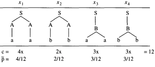
The distribution determined by the training corpus is known as the empirical distribution. For example, suppose we have a training corpus containing twelve trees of the four types from L(G1) shown in Figure 3, where

c(x)

is the count of how often the

X I X 2 X 3 X 4

S S S S

A A A A

a a b b a a b b

c = 4x 2x 3x 3x = 12

= 4/12 2/12 3/12 3/12

Figure 3

An empirical distribution. There are twelve parse trees of four distinct types.

tree (type) x appears in the corpus, and/3(.) is the empirical distribution, defined as:

c(x) N = c(x)

N

x

[image:5.468.37.300.424.537.2]

(6)

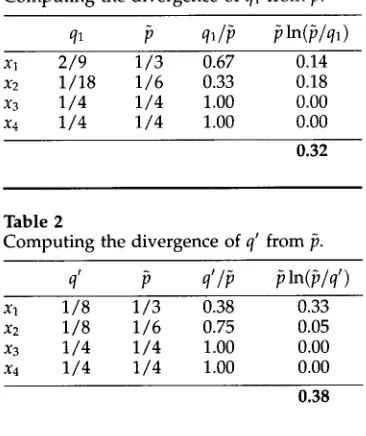
Table 1

Computing the divergence of ql from ft.

ql

~

ql/~

~ln(~/q,)

xl 2/9 1/3 0.67 0.14

x2 1/18 1/6 0.33 0.18

X 3 1/4 1/4 1.00 0.00

X4 1/4 1/4 1.00 0.00

0.32

Table 2

Computing the divergence of q' from ft.

q'

p

q'/~

filn(~/q')

xl 1/8 1/3 0.38 0.33

x2 1/8 1/6 0.75 0.05

x3 1/4 1/4 1.00 0.00

x4 1/4 1/4 1.00 0.00

0.38

is the Kullback-Leibler (KL) divergence, defined as:

D ( p l l q ) = In

x q(x)

The divergence between ~ a n d q at point x is the log of the ratio of ~(x) to

q(x).

The overall divergence b e t w e e n ~ a n d q is the average divergence, where the averaging is over tree (tokens) in the corpus; i.e., point divergences

In(~(x)/q(x))

are w e i g h t e d b y ~(x) a n d s u m m e d .

For example, let ql be, as before, the distribution d e t e r m i n e d b y m o d e l M1. Table 1 shows ql, P, the ratio ql ( X ) / ] ) ( X ) , a n d the weighted point divergence ~(x)

ln(~(x)/ql (x)).

The s u m of the fourth c o l u m n is the KL divergence D(~llql ) b e t w e e n ~ a n d ql. The third c o l u m n contains ql(x)/~(x) rather than

~(x)/ql (x)

so that one can see at a glance w h e t h e r

ql(x)

is too large (> 1) or too small (< 1). The total divergence D(~]lql ) = 0.32. One set of weights is better t h a n another if its divergence from the empirical distribution is less. For example, let us consider a different set of weights for g r a m m a r G1. Let M' be G1 w i t h weights ( 1 / 2 , 1 / 2 , 1 / 2 , 1 / 2 , 1 / 2 , 1 / 2 ) , a n d let q' be the probability distribution determined b y Mq Then the c o m p u t a t i o n of the KL divergence is as in Table 2. The fit for x2 improves, b u t that is more t h a n offset b y a poorer fit for Xl. The distribution ql is a better distribution t h a n

q', in

the sense that ql is more similar (less dissimilar) to the empirical distribution than q~ is.

One reason for adopting minimal KL divergence as a measure of goodness is that minimizing KL divergence maximizes likelihood. The likelihood of distribution q is the probability of the training corpus according to q:

L(q)

=

]-[

q(x)

x in training

=

I-[ q (x)~(~)

[image:6.468.50.233.77.295.2]

(7)

Since log is monotone increasing, maximizing likelihood is equivalent to maximizing log likelihood:

lnL(q)

=

y ~ c ( x ) l n q ( x )

x

=

The expression on the right-hand side is

- 1 / N

times the cross entropy of q with respect to ~, hence maximizing log likelihood is equivalent to minimizing cross entropy. Finally, D(~llq) is equal to the cross entropy of q less the entropy of ~, and the entropy of is constant with respect to q; hence minimizing cross entropy (maximizing likelihood) is equivalent to minimizing divergence.

2.2 The ERF Method

For stochastic context-free grammars, it can be shown that the ERF method yields the best model for a given training corpus. First, let us introduce some terminology and notation. With each rule i in a stochastic context-free grammar is associated a weight

fli and a functionj~(x) that returns the number of times rule i is used in the derivation

of tree x. For example, consider the tree in Figure 2, repeated here in Figure 4 for convenience: Rule 1 is used once and rule 3 is used twice; accordingly

fl(x)

= 1,

-"'"- ~1 .,Y°" S "'"',,

,.A x .." A.;i

'%•. • °." "%... o°•'

Figure 4

Rule applications in a parse tree.

f3(x) = 2, andy~(x) = 0 for i E {2,4,5,6}.

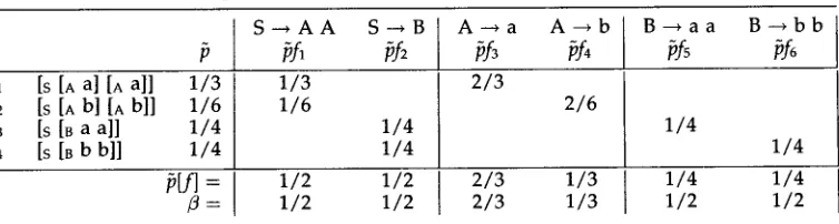
We use the notation p[yq to represent the expectation o f f under probability distribution p; that is, p[yq -- ~ x p(x)f(x). The ERF method instructs us to choose the weight

fli for rule i proportional to its empirical expectation ~[f;]. Algorithmically, we compute

the expectation of each rule's frequency, and normalize among rules with the same left-hand side.

(8)

Table 3

Parameter estimation using the ERF method.

Xl [S [A a] [A a]] 1/3

X2 [S [A b] [A b]] 1/6

x3 [s [B a a]] 1/4 x4 [s [B b b]] 1/4

=

f l =

S--* A A S--*B

/3fl /3f2

1/3 1/6

1/4 1/4

1/2 1/2

A--*a A ~ b

2/3

2/6

2/3 1/3

B ~ a a B ~ b b

pf5 pf6

1/4

1/4 1/4

1/2 1/2

defining distribution q, a n d

fl'

defining q~ is a n y set of weights such that q ~ q', then D(~]]q) < D(fii[q').

One m i g h t expect the best weights to yield D(fi[]q) = 0, b u t such is not the case. We have just seen, for example, that the best weights for g r a m m a r G1 yield distribution ql, yet D(/~]]ql) = 0.32 > 0. A closer inspection of the divergence calculation in Table 1 reveals that ql is sometimes less t h a n ~, b u t never greater than ~. Could we improve the fit b y increasing ql? For that matter, h o w can it be that ql is never greater t h a n fi? As probability distributions, ql and/3 should have the same total mass, namely, one. Where is the missing mass for ql?

The answer is of course that ql a n d /3 are probability distributions over

L(G1),

b u t not all of

L(G1)

appears in the corpus. Two trees are missing, a n d t h e y account for the missing mass. These two trees are given in Figure 5. Each of these trees has

S S

A A A A

I

a b b a

F i g u r e 5

The trees from

L(G1)

that are missing in the training corpus.

probability 0 according to ~ (hence they can be ignored in the divergence calculation), but probability 1/9 according to ql.

Intuitively, the problem is this: The distribution ql assigns too little weight to trees xl a n d x2, a n d too m u c h weight to the "missing" trees; call t h e m x5 a n d x6. Yet exactly the same rules are used in x5 a n d x6 as are used in xl a n d x2. Hence there is no w a y to increase the weight for trees Xl a n d x2, improving their fit to ~, w i t h o u t simultaneously increasing the weight for Xs a n d x6, m a k i n g their fit to ~ worse. The distribution ql is the best compromise possible.

To say it another way, our assumption that the corpus was generated b y a context- free g r a m m a r means that a n y context dependencies in the corpus m u s t be accidental, the result of sampling noise. There is indeed a d e p e n d e n c y in the corpus in Figure 3: in the trees where there are two A's, the A's always rewrite the same way. If the corpus was generated b y a stochastic context-free grammar, then this d e p e n d e n c y is accidental.

[image:8.468.57.434.83.184.2]

(9)

impossible for the resulting empirical distribution to m a t c h the distribution ql. But as the c o r p u s size increases, the fit b e t w e e n ~ a n d ql b e c o m e s ever better.

3. Attribute-Value Grammars

But w h a t if the d e p e n d e n c y in c o r p u s (3) is not accidental? W h a t if w e wish to a d o p t a g r a m m a r that imposes the constraint that b o t h A's rewrite the same way? We can i m p o s e such a constraint b y m e a n s of an attribute-value grammar.

We m a y formalize an attribute-value g r a m m a r as a context-free g r a m m a r w i t h attribute labels a n d p a t h equations. An e x a m p l e is the following g r a m m a r ; let us call it G2:

1. S--* I : A 2 : A /1 1) = / 2 1)

2. S --* I:B

3. A ~ l:a

4. A--* l:b

5. B --* l:a

6. B --* l:b

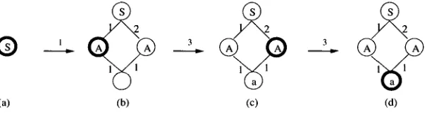
Figure 6 illustrates h o w a d a g is g e n e r a t e d f r o m G2. We begin in (a) w i t h a single

®

[image:9.468.35.338.342.425.2]

(a)

Figure 6

b D

(b) (c) (d)

Generating a dag. The grammar used is G2.

n o d e labeled w i t h the start category of G2, namely, S. A n o d e x is e x p a n d e d b y choosing a rule that rewrites the category of x. In this case, w e choose rule 1 to e x p a n d the root node. Rule 1 instructs us to create two children, b o t h labeled A. The e d g e to the first child is labeled 1 a n d the edge to the second child is labeled 2. The constraint (1 1) = (2 1) indicates that the 1 child of the 1 child of x is identical to the 1 child of the 2 child of x. We create an unlabeled n o d e to represent this g r a n d c h i l d of x a n d direct a p p r o p r i a t e l y labeled edges from the children, yielding (b).

We p r o c e e d to e x p a n d the n e w l y i n t r o d u c e d nodes. We choose rule 3 to e x p a n d the first A node. In this case, a child w i t h e d g e labeled 1 already exists, so w e use it rather than creating a n e w one. Rule 3 instructs us to label this child a, yielding (c). N o w w e e x p a n d the second A node. Again w e choose rule 3. We are instructed to label the 1 child a, b u t it already has that label, so w e d o not n e e d to d o anything. Finally, in (d), the only r e m a i n i n g n o d e is the b o t t o m - m o s t node, labeled a. Since its label is a terminal category, it does not n e e d to be e x p a n d e d , a n d w e are done.

(10)

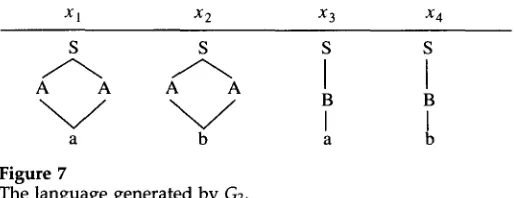
The language L(G2) is the set of dags produced by successful derivations, as shown in Figure 7. (The edges of the dags should actually be labeled with l ' s and 2's, but I

X 1 X 2 X 3 X 4

S S S S

A A A A

I

L

a b a b

Figure 7

The language generated by G2.

have suppressed t h e edge labels for the sake of perspicuity.)

3.1 AV G r a m m a r s and the ERF M e t h o d

Now we face the question of how to attach probabilities to grammar G2. The natural extension of the method we used for context-free grammars is the following: Associate a weight with each of the six rules of grammar G2. For example, let M2 be the model consisting of G2 plus weights (ill . . . /36) = (1/2,1/2, 2/3,1/3,1/2,1/2). Let

¢2(x)

be the weight that M2 assigns to dag x; it is defined to be the product of the weights of the rules used to generate x. For example, the weight ¢2(xl) assigned to tree xl of Figure 7 is 2/9, computed as in Figure 8. Rule 1 is used once and rule 3 is used twice;

Xl----

..""" S "'""..

:'i A'",, ..'"A ~i

,;. ",, .. ..:.

" . . • .' ~ 3 "~. i...'

Figure 8

Rule applications in a dag generated by G2. The weight of the dag is the product of the weights of rule applications.

hence ¢2(xl) =

fllfl3fl3

= 1 / 2 . 2 / 3 . 2 / 3 = 2/9.

Observe that ¢2(xa) =

fllfl 2,

which is to say,

fl/l(x,)fl/~(x,)

₁ ₃ _"Moreover, since fl0 1,

it does not hurt to include additional factors fl:(xl) for those i where y~(xl) = 0. That is, we can define the dag weight ¢ corresponding to rule weights fl = (ill . . . fin) generally as:

n

II

i = 1

The next question is how to estimate weights. Let us consider what happens when we use the ERF method. Let us assume a corpus distribution for the dags in Figure 7 analogous to the distribution in Figure 3:

X1 X2 X3 X4

--- 1/3 1/6 1/4 1/4 (1)

[image:10.468.53.310.87.186.2]

(11)

Table 4

Estimating the parameters of G2 using the ERF method.

xl 1/3 X2 1/6

X 3 1/4 X4 1/4 ~[;q =

f l =

1/3 1/6

1/4 1/4 1/2 1/2 1/2 1/2

2/3 2/6

2/3 1/3 2/3 1/3

1/4 1/4 1/4 1/4 1/2 1/2

3.2 Why the ERF Method Fails

But at this point a problem arises: ~2 is not a probability distribution. Unlike in the context-free case, the four dags in Figure 7 constitute the entirety of L(G2). This time, there are no missing dags to account for the missing probability mass.

There is an obvious "fix" for this problem: we can simply normalize 62. We might define the distribution q for an AV grammar with weight function ~b as:

q(X)=z~(X)

where Z is the normalizing constant:

xEL(G)

In particular, for ~2, w e have Z = 2/9 + 1/18 + 1/4 + 1/4 = 7/9. Dividing ~2 by 7/9 yields the ERF distribution:

Xl X2 X3 X4

q2(x)= 2/7 1/14 9/28 9/28

On the face of it, then, we can transplant the methods we used in the context-free case to the AV case and nothing goes wrong. The only problem that arises (@ not summing to one) has an obvious fix (normalization).

However, something has actually gone very wrong. The ERF method yields the best weights only under certain conditions that we inadvertently violated by chang-

ing L(G) and re-apportioning probability via normalization. In point of fact, we can

easily see that the ERF weights in Table 4 are

not the best weights for our example

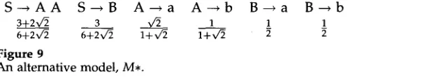
grammar. Consider the alternative model M* given in Figure 9, defining probability distribution q*.

S - * A A S--*B A - - * a A - ~ b B - - * a B - - * b

3-[-2v~ 3 x,~ 1 1 1

6q-2v/2 6+2v~ l + v ~ l + v ~ 2

Figure 9

An alternative model, M,.

[image:11.468.36.338.583.638.2]

(12)

side s u m to one. The reader can verify that ** sums to Z = 3+v~ a n d that q, is: ₃

X1 X2 X3 X4

q,(x) = 1/3 1/6 1/4 1/4

That is, q, = ]5. C o m p a r i n g q2 (the ERF distribution) a n d q, to ~, we observe that D(~llq2 ) = 0.07 but D(~llq, ) = O.

In short, in the AV case, the ERF weights do not yield the best weights. This means that the ERF m e t h o d does not converge to the correct weights as the corpus size increases. If there are genuine dependencies in the grammar, the ERF m e t h o d converges systematically to the w r o n g weights. Fortunately, there are m e t h o d s that do converge to the right weights. These are m e t h o d s that have been developed for r a n d o m fields.

4. Random Fields

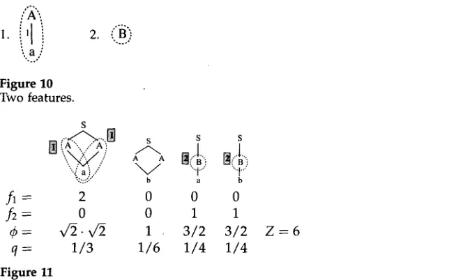
A r a n d o m field defines a probability distribution over a set of labeled graphs f~ called configurations. In our case, the configurations are the dags generated b y the grammar, i.e., f~ = L(G). The weight assigned to a configuration is the p r o d u c t of the weights assigned to selected features of the configuration. We use the notation:

,Ix)-- II

i

where fli is the weight for feature i a n d f/(.) is its frequency function, that is, fi(x) is the n u m b e r of times that feature i occurs in configuration x. (For most purposes, a feature can be identified w i t h its frequency function; I will not always m a k e a careful distinction b e t w e e n them.)

I use the term feature here as it is used in the machine learning a n d statistical pattern recognition literature, not as in the constraint g r a m m a r literature, w h e r e feature

is s y n o n y m o u s with attribute. In m y usage, dag edges are labeled w i t h attributes, not features. Features are rather like geographic features of dags: a feature is some larger or smaller piece of structure that occurs--possibly at more than one place---in a dag. The probability of a configuration (that is, a dag) is proportional to its weight, a n d is obtained b y normalizing the weight distribution.

q(x) = ½,(x) z = Gx a *(x)

If we identify the features of a configuration w i t h local trees equivalently, w i t h applications of rewrite r u l e s - - t h e r a n d o m field m o d e l is almost identical to the m o d e l we considered in the previous section. There are t w o important differences. First, we no longer require weights to s u m to one for rules w i t h the same left-hand side. Second, the m o d e l does not require features to be identified w i t h rewrite rules. We use the g r a m m a r to define the set of configurations f~ = L(G), b u t in defining a probability distribution over L(G), we can choose features of dags h o w e v e r we wish.

(13)

;X'.

- a :

, . . /

Figure 10

Two features.

s

: '' r / ~ - - . , ~ s s s

":::::::" b a b

fl---- 2 0 0 0

f2 = 0 0 1 1

4 = x / 2 - v ~ 1 3/2 3/2

q = 1/3 1/6 1/4 1/4

Figure 11

Z - - 6

The frequencies (number of instances) of features 1 and 2 in dags generated by G2, and the computation of dag weights ~ and dag probabilities q.

recreate the empirical distribution using fewer features than before. Intuitively, we need only use as many features as are necessary to distinguish among trees that have different empirical probabilities.

This added flexibility is welcome, but it does make parameter estimation more involved. Now we must not only choose values for weights, we must also choose the features that weights are to be associated with. We would like to do both in a way that permits us to find the best model, in the sense of the model that minimizes the Kullback-Leibler distance with respect to the empirical distribution. The IIS algorithm (Della Pietra, Della Pietra, and Lafferty 1995) provides a method to do precisely that.

5. Field Induction

In outline, the IIS algorithm is as follows:

1.

2.

.

4.

Start (t = 0) with the null field, containing no features.

Feature Selection. Consider every feature that might be added to field

Mt and choose the best one.

Weight Adjustment. Readjust weights for all features. The result is field

Mt+l.

Iterate until the field cannot be improved.

For the sake of concreteness, let us take features to be labeled subdags. In step 2 of the algorithm we do not consider every conceivable labeled subdag, but only the atomic (i.e., single-node) subdags and those complex subdags that can be constructed by combining features already in the field or by combining a feature in the field with some atomic feature. We also limit our attention to features that actually occur in the training corpus.

[image:13.468.30.367.51.252.2]

(14)

@@@@@

Figure 12

The atomic features arising in dags generated by G2.

Figure 13

Combining features to create more complex features.

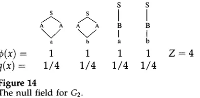
5.1 The N u l l Field

Field induction begins with the null field. With the c o r p u s w e h a v e b e e n assuming, the

null field takes the f o r m in Figure 14. N o dag x has a n y features, so ¢(x)

= I]i fl~(x)

is a

¢(x) --

q ( x ) =

Figure 14

S S

s s I I

A A A A B B

V V i i

a b a b

1 1 1 1

1 / 4 1 / 4 1 / 4 1 / 4

The null field for G2.

Z = 4

p r o d u c t of zero terms, a n d hence has value 1. As a result, q is the u n i f o r m distribution. The Kullback-Leibler d i v e r g e n c e D (/~ llq) is 0.03. The aim of feature selection is to choose a feature that reduces this divergence as m u c h as possible.

The astute reader will note that there is a p r o b l e m with the null field if

L(G)

is infinite. Namely, it is not possible to have a u n i f o r m probability mass distribution o v e r an infinite set. If each dag in an infinite set of dags is assigned a constant n o n z e r o probability e, t h e n the total probability is infinite, no m a t t e r h o w small e is. There are a couple of w a y s of dealing w i t h the problem. The a p p r o a c h that DD&L a d o p t is to assume a consistent prior distribution

p(k)

over g r a p h sizes k, a n d a family of r a n d o m fields qk representing the conditional probability

q(x I

k); the probability of a tree is then

p(k)q(x I k).

All the r a n d o m fields h a v e the same features a n d weights, differing only in their n o r m a l i z i n g constants.

I will take a s o m e w h a t different a p p r o a c h here. As sketched at the beginning of section 3, we can generate dags from an AV g r a m m a r m u c h as p r o p o s e d b y Brew and Eisele. If w e ignore failed derivations, the process of dag generation is c o m p l e t e l y analogous to the process of tree generation from a stochastic C F G - - i n d e e d , in the limiting case in w h i c h n o n e of the rules contain constraints, the g r a m m a r

is

a CFG. To obtain an initial distribution, we associate a w e i g h t with each rule, the weights for rules with a c o m m o n left-hand side s u m m i n g to one. The probability of a dag is p r o p o r t i o n a l to the p r o d u c t of weights of rules used to generate it. (Renormalization is necessary because of the failed derivations.) We estimate weights using the ERF method: w e estimate the w e i g h t of a rule as the relative f r e q u e n c y of the rule in the training corpus, a m o n g rules with the same left-hand side.

[image:14.468.54.251.244.341.2]

(15)

account of context dependencies that the ERF distribution fails to capture, incremen- tally improving the fit to the empirical distribution.

In this framework, a model consists of: (1) An AV grammar G whose purpose is to define a set of dags

L(G).

(2) A set of initial weights 0 attached to the rules of G. The weight of a dag is the product of weights of rules used in generating it. Discarding failed derivations and renormalizing yields the initial distribution

po(x).

(3) A set of features fl . . . .

,fn

with weights f l l . . . . , fin to define the field distribution

q(x) = ½Po(X) I-Ii fl?(x).

5.2 Feature S e l e c t i o n

At each iteration, we select a new feature f by considering all atomic features, and all complex features that can be constructed from features already in the field. Holding the weights constant for all old features in the field, we choose the best weight fl f o r f (how fl is chosen will be discussed shortly), yielding a new distribution qfi,/. The score for feature f is the reduction it permits in D(pl[qold), where qold is the old field. That is, the score for f is D(~llqold ) --

D(~llqfi,f ).

We compute the score for each candidate feature and add to the field that feature with the highest score.

To illustrate, consider the two atomic features a and B. Given the null field as old field, the best weight for a is fl = 7/5, and the best weight for B is fl ~- 1. This yields q and D(/S[~) as in Figure 15. The better feature is a, and a would be added to the field

~a

q~ filn

¢B

qB

~ln ~

Figure 15

S S

s s I I

A A A A B B

a b a b

1/3 1/6 1/4 1/4

7/5 1 7/5 1 Z = 24/5

7/24 5/24 7/24 5/24

0.04 -0.04 -0.04 0.05 D = 0.01

1 1 1 1 Z = 4

1/4 1/4 1/4 1/4

0.10 -0.07 0 0 D = 0.03

Comparing features, qa is the best (minimum-divergence) distribution that can be generated by adding the feature "a" to the field, and

qB

is the best distribution generable by adding the feature "B'.

if these were the only two choices.

[image:15.468.32.270.309.480.2]

(16)

5.3 Selecting the Initial Weight

DD&L show that there is a unique weight fl that maximizes the score for a new feature f (provided that the score for f is not constant for all weights). Writing q~ for the distribution that results from assigning weight fl to feature f , fl is the solution to the equation

q~[f] = ~[f] (2)

Intuitively, we choose the weight such that the expectation of f under the resulting new field is equal to its empirical expectation.

Solving equation (2) for fl is easy if

L(G)

is small enough to enumerate. Then the sum over

L(G)

that is implicit in qfl [f] can be expanded out, and solving for fl is simply a matter of arithmetic. Things are a bit trickier if

L(G)

is too large to enumerate. DD&L show that we can solve equation (2) if we can estimate qold[f = k] for k from 0 to the maximum value o f f in the training corpus. (See Appendix 1 for details.)

We can estimate qold[f = k] b y means of

random sampling.

The idea is actually rather simple: to estimate how often the feature appears in "the average dag," we generate a representative mini-corpus from the distribution qold and count. That is, we generate dags at random in such a w a y that the relative frequency of dag x is qold(X) (in the limit), and we count h o w often the feature of interest appears in dags in our generated mini-corpus.

The application that DD&L consider is the induction of English orthographic constraints, that is, inducing a field that assigns high probability to "English-sounding" words and low probability to non-English-sounding words. For this application, Gibbs sampling is appropriate. Gibbs sampling does not work for the application to AV grammars, however. Fortunately, there is an alternative random sampling method we can use: Metropolis-Hastings sampling. We will discuss the issue in some detail shortly.

5.4 Readjusting Weights

When a new feature is added to the field, the best value for its initial weight is chosen, but the weights for the old features are held constant. In general, however, adding the new feature may make it necessary to readjust weights for all features. The second half of the IIS algorithm involves finding the best weights for a given set of features. The method is very similar to the method for selecting the initial weight for a new feature. Let (fl . . . . ,

fin)

be the old weights for the features. We wish to compute "increments" (61,..., 6,) to determine a new field with weights (61fll,...,

6,ft,).

Consider the equation

qold[6/#fi] = p[f/] (3)

where

f#(x) = y'~if/(x)

is the total number of features of dag x. The reason for the factor 6 f# is a bit involved. Very roughly, we w o u l d like to choose weights so that the expectation offi under the

new

field is equal to/5[f/]. N o w qnew(X)

is:

qnew(X)

= ½polxl III6jfjl

J

1

H ~ x

= ~--~qold (X) • J

(17)

~j for all the features simultaneously, not just the weight ~i for feature i. We might consider approximating qnew[fi] by ignoring the normalization factor and assuming that all features have the same weight as feature i. Since

]-Ij 6~ (x)

= 6//'(x), we arrive at the expression on the left-hand side of equation (3).

One might expect the approximation just described to be rather poor, but it is proven in Della Pietra, Della Pietra, and Lafferty (1995) that solving equation (3) for

6i

(for each i) and setting the new weight for feature i to

~ifli

is guaranteed to improve the model. This is the real justification for equation (3), and the reader is referred to Della Pietra, Della Pietra, and Lafferty (1995) for details.

Solving (3) yields improved weights, but it does not necessarily immediately yield the globally best weights. We can obtain the globally best weights by iterating. Set

fli - 6ifli,*

for all i, and solve equation (3) again. Repeat until the weights no longer

change.

As with equation (2), solving equation (3) is straightforward if

L(G)

is small enough to enumerate, but not if

L(G)

is large. In that case, we must use random sampling. We generate a representative mini-corpus and estimate expectations by counting in the mini-corpus. (See Appendix 2.)

5.5 Random Sampling

We have seen that random sampling is necessary both to set the initial weight for features under consideration and to adjust all weights after a new feature is adopted. Random sampling involves creating a corpus that is representative of a given model distribution

q(x).

To take a very simple example, a fair coin can be seen as a method for sampling from the distribution q in which

q(H)

= 1/2,

q(T)

= 1/2. Saying that a corpus is representative is actually not a comment about the corpus itself but the method by which it was generated: a corpus representative of distribution q is one generated by a process that samples from q. Saying that a process M samples from q is to say that the empirical distributions of corpora generated by M converge to q in the limit. For example, if we flip a fair coin once, the resulting empirical distribution over (H, T) is either (1, 0) or (0,1), not the fair-coin distribution (1/2,1/2). But as we take larger and larger corpora, the resulting empirical distributions converge to (1/2,1/2). An advantage of SCFGs that random fields lack is the transparent relationship between an SCFG defining a distribution q and a sampler for q. We can sample from q by performing stochastic derivations: each time we have a choice among rules expanding a category X, we choose rule X --* ~i with probability

fli,

where

fli

is the weight of rule

X-- G*

N o w we

can

sample from the initial distribution p0 by performing stochastic derivations. At the beginning of Section 3, we sketched how to generate dags from an AV grammar G via nondeterministic derivations. We defined the initial distribution in terms of weights ~ attached to the rules of G. We can convert the nondeterministic derivations discussed at the beginning of Section 3 into stochastic derivations by choosing rule X --* ~i with probability ~i when expanding a node labeled X. Some derivations fail, but throwing away failed derivations has the effect of renormalizing the weight function, so that we generate a dag x with probability p0 (x), as desired.

The Metropolis-Hastings algorithm provides us with a means of converting the sampler for the initial distribution

po(x)

into a sampler for the field distribution

q(x).

Generally, let p(.) be a distribution for which we have a sampler. We wish to construct a sample xl . . . xN from a different distribution q(.). Assume that items xl . . . . , x, are already in the sample, and we wish to choose xn+l. The sampler for p(.)

proposes a

(18)

from p(.)--but rather we make a stochastic decision whether to accept the proposal y or reject it. If we accept y, it is added to the sample (Xn+l = y), and if we reject y, then

Xn

is repeated (Xn+l =

xn).

The acceptance decision is made as follows: If

p(y)

> q(y), then y is overrepresented among the proposals. We can quantify the degree of overrepresentation as

p(y)/q(y).

The idea is to reject y with a probability corresponding to its degree of overrepresentation. However, we do not consider the absolute degree of overrepresentation, but rather the degree of overrepresentation relative to x,. (If y and

Xn

are equally overrepresented, there is no reason to reject y in favor of xn.) That is, we consider the value

p(y)/q(y) _ p(y)q(xn)

r =

p(x,)/q(xn)

p(xn)q(y)

If r <_ 1, then y is underrepresented relative to x,, and we accept y with probability one. If r > 1, then we accept y with a probability that diminishes as r increases: specifically, with probability

1/r.

In brief, the acceptance probability of y is

A(y

] x,) = min(1,1/r). It can be shown that proposing items with probability p(.) and accepting them with probability A(. ] x,) yields a sampler for q(.). (See, for example, Winkler [1995]). 2

The acceptance probability

A(y ] xn)

reduces in our case to a particularly simple form. If r < 1 then

A(y

] x) = 1. Otherwise, writing ~b(x) for the "field weight"

[Ii fl~lxl,

we have:

A(y]xn)

-~ z-I~(Y)P°(Y)P°(X")

Z-'d~(x.)po(x,)po(y) (4)

(~(y ) / dp( Xn )

6. Final Remarks

In summary, we cannot simply transplant CF methods to the AV grammar case. In particular, the ERF method yields correct weights only for SCFGs, not for AV grammars. We can define a probabilistic version of AV grammars with a correct weight-selection method by going to random fields. Feature selection and weight adjustment can be accomplished using the IIS algorithm. In feature selection, we need to use random sampling to find the initial weight for a candidate feature, and in weight adjustment we need to use random sampling to solve the weight equation. The random sampling method that DD&L used is not appropriate for sets of dags, but we can solve that problem by using the Metropolis-Hastings method instead.

Open questions remain. First, random sampling is notorious for being slow, and it remains to be shown whether the approach proposed here will be practicable. I expect practicability to be quite sensitive to the choice of grammar--the more the grammar's

2 The Metropolis-Hastings acceptance probability is usually given in the form

( ly ly,

A(y [ x) = min 1,~r(x)g(x,y)]

in which 7r is the distribution we wish to sample from (q, in our notation) and g(x, y) is the proposal probability: the probability that the input sampler will propose y if the previous configuration was x. The case we consider is a special case in which the proposal probability is independent of x: the proposal probability g(x, y) is, in our notation, p(y).

(19)

distribution diverges from the initial context-free approximation, the more features will be necessary to "correct" it, and the more random samplingwill be called on.

A second issue is incomplete data. The approach described here assumes complete data (a parsed training corpus). Fortunately, an extension of the method to handle incomplete data (unparsed training corpora) is described in Riezler (1997), and I refer readers to that paper.

As a closing note, it should be pointed out explicitly that the random field techniques described here can be profitably applied to context-free grammars, as well. As Stanley Peters nicely put it, there is a distinction between

possibilistic

and

probabilistic

context-sensitivity. Even if the language described by the grammar of interest--that is, the set of possible trees---is context-free, there may well be context-sensitive statistical dependencies. Random fields can be readily applied to capture such statistical dependencies whether or not

L(G)

is context-sensitive.

Appendix A: Initial Weight Estimation

In the feature selection step, we choose an initial weight fl for each candidate feature f so as to maximize the

gain

G = D(/~llqold ) --

D(~[Iqf,~ )

of adding f to the field. It is actually more convenient to consider log weights c~ = In ft. For a given feature f, the log weight 6 that maximizes gain is the solution to the equation:

where q~ is the distribution that results from adding f to the field with log weight ~. This equation can be solved using Newton's method. Define

= # [ ; q - q [jq (5)

To find the value of c~ for which F(c~) = 0, we begin at a convenient point s0 (the "null" weight c~0 = 0 recommends itself) and iteratively compute:

F(~t)

(6)

t+l =

Della Pietra, Della Pietra, and Lafferty (1995) show that F'(oq) is equal to the negative of the variance o f f under the new field, which I will write - V ~ If].

To compute the iteration (6) we need to be able to compute

F(o~t)

and

F'(oq).

For

F(c~t) we require ~[f] and q~[f], and F'(~t) can be expressed

a s q , ~ [ f ] 2 _ q~[f2]./~[f] is simply the average value of f in the training corpus. The remaining terms are all of the form q~ IF]. We can re-express this expectation in terms of the old field qold:

x

Y~xfr(x)e~f(X)qold(X)

Y~x e~f(X)qold (X)

qold

[fre~f]

qold [e c~f ]

(20)

( 1 / N ) s r ( a ) , where:

sr( ) = ~fr(zk)e°~f(zk)

k

: ~ c o u n t k [ f ( Z k ) = u ] u r e c~u u

This yields:

q~,[f~]_ s~(a)

so(a)

and the Newton iteration (6) reduces to:

~ t + l z ~ t +

-

SO( OLt )S2 ( OLt ) -- S l ( O~t ) 2

To compare candidates, we also need to know the gain D(p]lqold ) -D(/~]]q6) for each candidate. This can be expressed as follows (Della Pietra, Della Pietra, and Lafferty 1995):

G(f,&) = p [ f ] l n & - lnqold[e 6f]

~[f] ln& -- lns0(&) + InN

Putting everything together, the algorithm for feature selection has the following form. The array E[J] is assumed to have been initialized with the empirical expectations

P i l l .

procedure SelectFeature 0 begin

Fill array C[f, u] = countk[f(zk) = u] by sampling from old field

~-- 0, g +-- none

for each f in candidates do c~ ,~-- 0

until ~ is accurate enough do

SO +--- S1 +-- S2 ~-- 0 for u from 0 to Umax do

x *-- C[f, u]e ~u

S0 + - - S 0 q - X Sl ~ SO q- XU 82 +-- S0 q- XU 2

end

Oz ~--- Oz q- ~

end

G +- aE[f] - I n s o + InN

if G > G then G ~-- G, g *--f, & ~-

(21)

Appendix B: Adjusting Field Weights

The procedure for adjusting field weights has m u c h the same structure as the procedure for choosing initial weights. In terms of log weights, we wish to c o m p u t e increments (61 . . . 5,) such that the n e w field, with log weights (c~1 + 61 . . . O~n q- 6n) has a lower divergence than the old field (c~1 .. . . . C~n). We choose each 6i as the solution to the equation:

p[fi] = qold[fie 6if~ ] ¢i

Again, we use N e w t o n ' s method. We wish to find 5 such that

Fi(6)

= 0, where:

F i ( 6 ) = ]9[fi] _{-- qold[fie ]}6f#

As Della Pietra, Della Pietra, and Lafferty (1995) show, the first derivative is:

FI( 6 ) = --qold[fif#e 6y ]*

We see that the expectations we need to compute b y sampling from qold are of form qold

[fifie~f@

We generate a r a n d o m sample (Zl . . . ZN) a n d define:

Sr(i, 6) = ~ f i ( Z k ) f # ( z k ) r e 6f*(zk) k

= y ~ y ~ c o u n t k [ f i ( Z k ) = U

Af#(zk)

= m ] u m r e 6m

= ~-~mre 6m ~

fi(Zk)

m k[/:#(Zk)=m

As we generate the sample we u p d a t e the array

C[i, m] = Y~k[f~

(zk)=mfi(Zk)"

W e estimate

qold[fifie ~f"]

as the average value

of rifle ~f*

in the sample, namely,

(1/N)sr(i,6).

This permits us to c o m p u t e

Fi(6)

and

FI(6 ).

The resulting N e w t o n iteration is:

6t+l = 6t -{-

Nf~[fi] - so(i, 6t)

s1(i, 6)

The estimation procedure is:

procedure

AdjustWeights

(Oz I . . . ~ n ) begin until

the field converges

do

Fill array C[i, m]

by sampling from q~

for i from 1 to n 6+--0

until 6

is sufficiently accurate

do

So +'- Sl *--- 0

for m from 0 to n/max do

x ~-- C[i, m]e &'

So +-- SO q- X Sl ~ Sl Jr- x m

end

(22)

end

OL i +-- OL i q - ¢~

end end

r e t u r n ( a l . . . . , an) end

Acknowledgments

This work has greatly profited from the comments, criticism, and suggestions of a number of people, including Yoav Freund, John Lafferty, Stanley Peters, Hans

Uszkoreit, and members of the audience at talks I gave at Saarbrficken and Tfibingen. Michael Miller and Kevin Mark introduced me to random fields as a way of dealing with context-sensitivities in language, planting the idea that led (much later) to this paper. Finally, I would especially like to thank Marc Light and Stefan Riezler for extended discussions of the issues

addressed here and helpful criticism of my first attempts to present this material. All responsibility for flaws and errors of course remains with me.

References

Brew, Chris. 1995. Stochastic HPSG. In

Proceedings of EACL-95.

Della Pietra, Stephen, Vincent Della Pietra, and John Lafferty. 1995. Inducing features of random fields. Technical Report CMU-CS-95-144, CMU.

Eisele, Andreas. 1994. Towards probabilistic extensions of constraint-based grammars. Technical Report Deliverable R1.2.B, DYANA-2.

Gibbs, W. 1902. Elementary Principles of Statistical Mechanics. Yale University Press, New Haven, CT.

Mark, Kevin, Michael Miller, Ulf Grenander, and Steve Abney. 1992. Parameter estimation for constrained context-free language models. In Proceedings of the Fifth Darpa Workshop on Speech and Natural

Language, San Mateo, CA. Morgan

Kaufman.

Riezler, Stefan. 1996. Quantitative constraint logic programming for weighted

grammar applications. Talk given at LACL, September.

Riezler, Stefan. 1997. Probabilistic constraint logic programming. Arbeitspapiere des Sonderforschungsbereichs 340, Bericht Nr. 117, Universit~it Tfibingen.