DETERMINATION OF OPTIMAL RESERVE INVENTORY BETWEEN MACHINES IN SERIES WITH
STOCHASTIC BREAKDOWN DURATIONS HAVING SCBZ PROPERTY
Govindhan M and Elangovan R
Department of Statistics, Annamalai University, Annamalai Nager-608002, Tamil Nadu, India
A R T I C L E I N F O A B S T R A C T
The determination of optimal inventory theory several variations of inventory problem are discussed. The objective is to derive the optimal re-order level or optimal stock level. In this paper the optimal reserve inventory between two machines in series attempted.
The output of machine M1 is the input for machine and . Whenever the breakdown
of the machine M1 is at fault i.e not working, then the machine and may go to an
idle stage. The ideal time of and is very expensive and hence to prevent the ideal time of and a reserve inventory is maintained in between M1 and , .
The breakdown durations of machine M1 is a random variable. This random variable is
assumed to possess the called Setting the Clock Back to Zero (SCBZ) property for two random variables namely the breakdowns duration and interarrival times between repairs of M1 the optimal reserve inventory size is obtained. Numerical illustration also substantiated.
INTRODUCTION
In many manufacturing industries the production of products is in series of machines. The optimal reserve between the systems, namely, the system that produces the input and the system that consumes the input obtained from the previous system. If various manufacturing processes operate successively, then in the case of breakdown of one at some stage can affect the entire system. Hence stocking points of inventory are created between adjacent stages so as to achieve a certain degree of independence in operating the stages. In the present model the optimal size of the reserve of raw material to be maintained in between two machines in series is found out. A system in which there are two machine M1 is in first stage and in the second stage there are two machines and is considered. The output of machine M1 is the input for machine and . Whenever the breakdown of the machine M1 is at fault i.e not working, then the machine and may go to an idle stage. The ideal time of and is very expensive and hence to prevent the ideal time of and a reserve inventory is maintained in between M1 and , . The breakdown durations of machine M1 is a random variable. This random variable is assumed to possess the so called Setting the Clock Back to Zero (SCBZ) property for two random variables namely the breakdowns and interarrival times between repairs of M1 the optimal reserve inventory size is obtained. Numerical illustration also substantiated.
The determination if the optimal size of reserve inventory between M1 and M2 has been discussed by many authors, the have introduced the property called Setting the Clock Back to Zero Property (SCBZ property) RajaRao and Talwalkar (1990). The model is derived for optimal reserve between two machines with repair time having SCBZ (Setting the Clock Back to Zero) property has been discussed by Sachithananatham, et.al. (2006). The optimal reserve inventory between two machines under SCBZ property of inter-arrival times between breakdowns has been discussed by Srinivasan, et.al. (2007). The expected time to recruitment when threshold distribution has SCBZ property has been discussed by Sathiyamoorthi, and Parthasarathy, (2003). The basic model involving two machines in series and the determination of optimal reserve between two machines has been discussed by Hansman (1962). An extension of model is carried out in this paper.
Notations
S -Level of reserve inventory
X0 - A continuous random variable which denotes the repair time of M1 with p.d.f is g(.)
with c.d.f G (.)
µ - mean time interval between the successive breakdowns of machine M1
- A random variable which denotes the duration of breakdown / repair time M1 and it has p.d.f g(.) with c.d.f G(.) and ~exp ( ).
International Journal of Current Advanced Research
ISSN: O: 2319-6475, ISSN: P: 2319 – 6505, Impact Factor: SJIF: 5.995
Available Online at www.journalijcar.org
Volume 6; Issue 8; August 2017; Page No. 5146-5150
DOI: http://dx.doi.org/10.24327/ijcar.2017.5150.0661
Article History:
Received 10th May, 2017 Received in revised form 5th
June, 2017 Accepted 16th July, 2017 Published online 28th August, 2017
Research Article
Copyright©2017 Govindhan M and Elangovan R. This is an open access article distributed under the Creative Commons Attribution License, which permits unrestricted use, distribution, and reproduction in any medium, provided the original work is properly cited.
Key words:
System in Series, Breakdown Duration, SCBZ Property, Optimal Reserve,
*Corresponding author: Govindhan M
h - Inventory holding cost per unit time d1 - Cost per unit of idle time of machine d2 - Cost per unit of idle time of machine r1 -Consumption rate per unit time of machine r2 - Consumption rate per unit time of machine
Assumptions
1.The output at the M1 which is a semi finished products is the input for and
2.Machine M1 undergoes breakdown for a random duration 3.Whenever M1 undergoes a breakdown, then the supply of
the raw material for and is from the reserve inventory
4.The consumption rate of and are fixed Constants 5.The breakdown time of M1 is a random variable
Results I
In this model two machines M1 and and in series is considered and the optimal value of reserve inventory between M1 and and for the system given above in the introduction is discussed.
if T is a random variable denoting idle time of machines and during a repair time of machine M1 will be noted that
=
< +
−
+ > +
As there are breakdowns per unit time, the expected cost
per unit time becomes
( ) =ℎ + +
µ − +
∞
( ) . . . (1)
To obtain optimal reserve inventory S,
To find ( )= 0, it may be observed that the differentiating (1) both sides w.r.t S by using the Leibnitz rule of differentiation of integral, we get,
( )
=ℎ −
µ( ) ∫ ( )
∞
. . . (2)
Thus, ( )
=ℎ − +
µ( + ) 1− + . . . (3)
To determine the optimal reserve inventory level , it is required to solve
( )
= 0 ⋯(4)
Therefore, the optimal reserve inventory level is given as,
+ = 1−
( + ) ℎ
( + ) ⋯(5)
Results II
In this model it is assumed that the breakdown duration of machine M1 which is denoted as a random variable with p.d.f g(t) is such that satisfies the Setting the Clock Back to Zero (SCBZ) property. For detailed Study of the SCBZ
property, one refers to Raja Rao and Talwalker (1990). According to this property the probability distribution of the random variable has a parametric change when ≥ ,
where is a truncation point of random variable X. The distribution remains the same except for the fact that the parameter changes from to . it may be stated that f(X, ) → f ( X, ) whenever X > X0.
A condition which ensure the existence of the SCBZ property for any distribution is that
(X + X , )
(X, ) = S(X, )
In the present model it is assumed that the breakdown duration which is a random variable has a p.d.f which satisfies SCBZ property.
The random variable follows g( , ) if < X , and it follows g( , ) if ≥ where is the truncation point and G(.) is the c.d.f of .
Now the expected total cost can be represented as
( ) =ℎ +( + )
⎣ ⎢ ⎢ ⎡
g( , )
( )
+ g( , )
∞
⎦ ⎥ ⎥ ⎤
⋯(6)
Special Case
Consider the following p.d.f.
( ) = ( ≤ )
>
It can be shown that g( ) satisfies the SCBZ property.
Result I
When lies before X0, (i.e.,) ≤ , where S is the initial reserve inventory level Kept and it is an assumed value.
( ) =ℎ +( + )
⎣ ⎢ ⎢ ⎡
−
+ ( )
( )
+ −
+ ( )
∞
⎦ ⎥ ⎥ ⎤
⋯(7)
To find ( ) = ,
h +
⎣ ⎢ ⎢ ⎡
⎩ ⎨ ⎧
−
+ ( ) + − + ( )
∞
( ) ⎭
⎬ ⎫
⎦ ⎥ ⎥ ⎤
Let we have
I = −
+ ( )
( )
⋯(8)
And
I = −
+ ( )
∞
⋯(9)
Determination of Optimal Reserve Inventory Between Machines in Series with Stochastic Breakdown Durations Having Scbz Property
I = 0 − 1
+ + + , +
−1
+ ( )
( )
=− 1
+ ( )
=− 1
+ ( , )− ( + ) ⋯(10)
therefore, we have
= −1
+ ( )
∞
=− 1
+ ( )
∞
= −1
+ ̅ ( , ) ⋯(11)
where
̅ ( , ) = ( ≥ )
( )
=ℎ+ + − + ( ) + − + ( )
∞
( ) = 0
ℎ − +
( + ) ( , )− + + ̅ ( , ) = 0
( , )−
+ + ̅ ( , ) =
ℎ ( + )
+ ⋯(12)
G( , )−G
+ , = ( ) = ( )
=
= −
= − ⋯(13)
Now we consider,
̅ ( , ) = ( )
∞
= ( )
∞
= ( )
−
∞
= ( )
=
= ( )
= … (14)
Substitute (13) and (14) in equation (12).
G( , )−G
+ , + ̅ ( , ) =
ℎ ( + )
+
− + =ℎ ( + )
+
=ℎ ( + )
+ … (15)
The above equation (15) by taking log on both sides becomes,
−
+ =
ℎ ( + )
+
Therefore, the optimal reserve inventory level is given as,
=
ℎ ( + )
+ ( + )
− ⋯(16)
Result (ii)
When falls after X0 i.e >
( ) =ℎ + +
⎣ ⎢ ⎢ ⎡
( −
+
∞
) ( )
⎦ ⎥ ⎥ ⎤
Now taking,
( ) = 0
ℎ+ + − + ( ) = 0
( ) = 0
ℎ − +
( + ) − + ( ) = 0
( ) = ℎ ( + )
+
1− = ( ) ⋯(17)
( ) =
∞
ℎ ( + )
+
[ ( ) ] =
∞
ℎ ( + )
( ) [ ] = ℎ ( + )
+
( )
−
∞
= ℎ ( + ) +
( ) = ℎ ( + )
+
= ℎ ( + )
+
( ) … (18)
The above equation (18) by taking log on both sides becomes,
− log = ( ) + ( − )
Therefore, the optimal reserve inventory level
=
ℎ ( + )
+ + ( − ) ( + )
− log ⋯(19)
The optimal valve of can be obtained by using (16) and (19).
=
⎩ ⎪ ⎨ ⎪
⎧ ℎ( ++ ) ( + )
− + ≤
ℎ ( + )
+ + ( − ) ( + )
− log + >
Numerical Illustration
The variation in the values of consequent to the changes in parameter h, , , , , the demand rate , , and ideal
time cost , , have been taking numerical illustration. The table and corresponding graphs are given as.
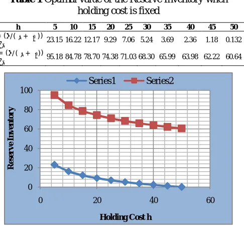
If the value of inventory holding cost h increases the optimal inventory size namely decreases therefore a smaller reserve inventory will increase the profit, in both the cases namely ( /( + )) ≤ and ( /( + )) > . This is observed in Table 1 and Fig 1.
If the value of d1 which denotes the shortage cost due to inadequate suppley to machine increases then as increasing the reserve inventory is suggested in both the cases namely ( /( + )) ≤ and ( /( + )) > and this is a indicated in Table 2 and Fig 2.
If the value of d2 which the shortage cost arising due to machine increase then an increase in the values of is also observed and therefore if the shortage cost of machine 2 increases a higher level of reserve inventory is suggested in both the cases namely ( /( + )) ≤ and ( /( +
)) > . It is observed in Table 3 and Fig 3.
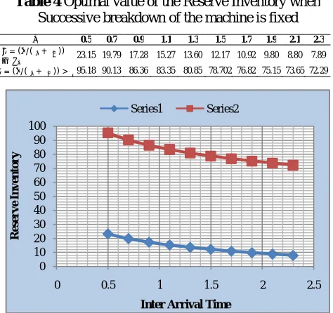
If the values of which is the average inter arrival time between the successive failure of machine M1 increases then a smaller reserve inventory is suggested in both the cases namely ( /( + )) ≤ and ( /( + )) > . This is obsevrved in Table 4 and Fig 4.
Table 1 Optimal value of the Reserve Inventory when holding cost is fixed
h 5 10 15 20 25 30 35 40 45 50
= ( /( + ))
≤ 23.15 16.22 12.17 9.29 7.06 5.24 3.69 2.36 1.18 0.132
= ( /( + ))
> 95.18 84.78 78.70 74.38 71.03 68.30 65.99 63.98 62.22 60.64
Fig 1 Optimal value of s when holding cost is fixed 0
20 40 60 80 100
0 20 40 60
R
e
se
r
v
e
I
n
v
e
n
to
r
y
Holding Cost h
Series1 Series2
Table 2 Optimal value of the Reserve Inventory when shortage cost for is fixed
d1 180 190 200 210 220 230 240 250 260 270
= ( /( + )) ≤ 23.15 23.418 23.671 23.918 24.159 24.394 24.62 24.84 25.06 25.28
= ( /( + )) > 95.18 95.570 95.950 96.321 96.682 97.035 97.38 97.71 98.04 98.36
Fig 2 Optimal value of ̂ when shortage cost for is fixed
Table 3 Optimal value of the Reserve Inventory when shortage cost for is fixed
d2 200 210 220 230 240 250 260 270 280 290
= ( /( + ))
≤ 23.15 23.418 23.671 23.918 24.159 24.394 24.62 24.84 25.06 25.28
= ( /( + ))
> 95.18 95.570 95.950 96.321 96.682 97.035 97.38 97.71 98.04 98.36
Fig 3 Optimal value of ̂ when shortage cost for is fixed
20 40 60 80 100 120
200 220 240 260 280 300
R
es
er
v
e
In
v
en
to
ry
Shortage Cost
Determination of Optimal Reserve Inventory Between Machines in Series with Stochastic Breakdown Durations Having Scbz Property
CONCLUSIONS
The following conclusions are drawn on the basis of the numerical illustration that has been worked out for this model.
1. As the value of inventory holding cost h increases the optimal inventory size namely decreases therefore a smaller reserve inventory will increase in both the cases namely ( /( + )) ≤ and ( /( +
)) > .
2. If the value of d1 which denotes the shortage cost due to inadequate supply to machine has an increase then an increase in the reserve inventory is suggested in both the cases namely ( /( + )) ≤ and ( /( + )) > .
3. If the value of d2 which the shortage cost arising due to machine increases an increase the value of is also observed in both the cases namely ( /( + )) ≤ and ( /( + )) > .
4. If the value of which is the average inter arrival time between the successive failure is of machine M1 increases a smaller reserve inventory is suggested in both the cases namely ( /( + )) ≤ and ( /( + )) > .
Reference
1. Sachithananatham. S, Ganesan. V, and
Sathiyamoorthi.R (2006), Optimal Reserve between Two machines with repair time having SCBZ property,
Bulletin of Pure and Applied Sciences, Vol.25E, No.2,
pp 487-497, 2006.
2. Srinivasan, S., Sulaiman, A., and Sathiyamoorthi. R. (2007), Optimal Reserve Inventory between Two Machines Under SCBZ Property of Interarrival Times between Breakdowns, Ultra Scientist of Physical
Sciences, Vol.19, No.2, pp 261-266, 2007.
3. Sathiyamoorthi, R. and Parthasarathy, S (2003), On the expected time to recruitment when thereshold distribution has SCBZ property, International Journal
of Management and Systems, Vol.19, No.3, pp
233-240, 2003.
4. Hanssman F (1962), Operation Research in Production and Inventory Control, John Wiley and Sons, Inc New York, 1962 pp 45-46.
5. RajaRao, B (1990). and Talwalkar, Setting the Clock Back to Zero Property of a Family of Life Distributions, Journal of Statistical Planning and
Inference, Vol.24, pp 347-352, 1990.
Table 4 Optimal value of the Reserve Inventory when Successive breakdown of the machine is fixed
0.5 0.7 0.9 1.1 1.3 1.5 1.7 1.9 2.1 2.3
= ( /( + ))
≤ 23.15 19.79 17.28 15.27 13.60 12.17 10.92 9.80 8.80 7.89
= ( /( + )) > 95.18 90.13 86.36 83.35 80.85 78.702 76.82 75.15 73.65 72.29
Fig 4 Optimal value of ̂ when Successive breakdown of the machine is fixed
0 10 20 30 40 50 60 70 80 90 100
0 0.5 1 1.5 2 2.5
R
e
se
r
v
e
I
n
v
e
n
to
r
y
Inter Arrival Time
Series1 Series2
How to cite this article:
Govindhan M and Elangovan R (2017) 'Determination of Optimal Reserve Inventory Between Machines in Series with Stochastic Breakdown Durations Having Scbz Property', International Journal of Current Advanced Research, 06(08), pp. 5146-5150. DOI: http://dx.doi.org/10.24327/ijcar.2017.5150.0661