Interpreting the neural code with formal concept analysis

Interpreting the Neural Code with

Formal Concept Analysis

Dominik Endres, Peter F¨oldi´ak

School of Psychology,University of St. Andrews KY16 9JP, UK

{dme2,pf2}@st-andrews.ac.uk

Abstract

We propose a novel application of Formal Concept Analysis (FCA) to neural de-coding: instead of just trying to figure out which stimulus was presented, we demonstrate how to explore the semantic relationships in the neural representation of large sets of stimuli. FCA provides a way of displaying and interpreting such relationships via concept lattices. We explore the effects of neural code sparsity on the lattice. We then analyze neurophysiological data from high-level visual corti-cal area STSa, using an exact Bayesian approach to construct the formal context needed by FCA. Prominent features of the resulting concept lattices are discussed, including hierarchical face representation and indications for a product-of-experts code in real neurons.

1

Introduction

Mammalian brains consist of billions of neurons, each capable of independent electrical activity. From an information-theoretic perspective, the patterns of activation of these neurons can be un-derstood as the codewords comprising the neural code. The neural code describes which pattern of activity corresponds to what information item. We are interested in the (high-level) visual system, where such items may indicate the presence of a stimulus object or the value of some stimulus at-tribute, assuming that each time this item is represented the neural activity pattern will be the same or at least similar.Neural decodingis the attempt to reconstruct the stimulus from the observed pat-tern of activation in a given population of neurons [1, 2, 3, 4]. Popular decoding quality measures, such as Fisher’s linear discriminant [5] or mutual information [6] capture how accurately a stimu-lus can be determined from a neural activity pattern (e.g., [4]). While these measures are certainly useful, they tell us little about the structure of the neural code, which is what we are concerned with here. Furthermore, we would also like to elucidate how this structure relates to the represented information items, i.e. we are interested in the semantic aspects of the neural code.

We would also like to be able to represent how the relationship between sets of active neurons trans-lates into the corresponding relationship between the encoded stimuli. These observations can be formalized by the well developed branch of mathematical order theory calledFormal Concept Anal-ysis(FCA) [8, 9]. In FCA, data from a binary relation (orformal context) is represented as a concept lattice. Each concept has a set offormal objectsas an extent and a set offormal attributesas an in-tent. In our application, the stimuli are the formal objects, and the neurons are the formal attributes. The FCA approach exploits the duality of extensional and intensional descriptions and allows to visually explore the data in lattice diagrams. FCA has shown to be useful for data exploration and knowledge discovery in numerous applications in a variety of fields [10, 11].

We give a short introduction to FCA in section 2 and demonstrate how the sparseness (or denseness) of the neural code affects the structure of the concept lattice in section 3. Section 4 describes the generative classifier model which we use to build the formal context from the responses of neurons in the high-level visual cortex of monkeys. Finally, we discuss the concept lattices so obtained in section 5.

2

Formal Concept Analysis

Central to FCA[9] is the notion of the formal contextK:= (G, M, I), which is comprised of a set of formal objectsG, a set of formal attributesMand a binary relationI⊆G×Mbetween members ofGandM. In our application, the members ofGare visual stimuli, whereas the members ofM

are the neurons. If neuronm ∈ M responds when stimulusg ∈ Gis presented, then we write

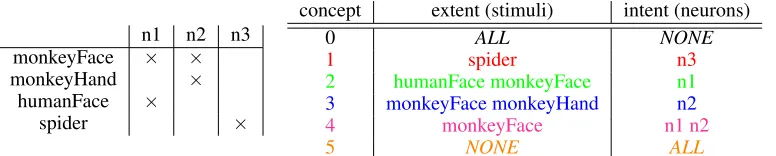
(g, m)∈IorgIm. It is customary to represent the context as a cross table, where the row(column) headings are the object(attribute) names. For each pair(g, m) ∈ I, the corresponding cell in the cross table has an ”x”. Table 1, left, shows a simple example context.

n1 n2 n3 monkeyFace × ×

monkeyHand ×

humanFace ×

spider ×

concept extent (stimuli) intent (neurons)

0 ALL NONE

1 spider n3

2 humanFace monkeyFace n1

3 monkeyFace monkeyHand n2

4 monkeyFace n1 n2

5 NONE ALL

Table 1: Left: a simple example context, represented as a cross-table. The objects (rows) are 4 visual stimuli, the attributes (columns) are 3 (hypothetical) neurons n1,n2,n3. An ”x” in a cell indicates that a stimulus elicited a response from the corresponding neuron. Right: the concepts of this context. Concepts are lectically ordered [9]. Colors correspond to fig.1.

Define the prime operator for subsetsA⊆GasA0={m∈M|∀g∈A:gIm}i.e.A0is the set of all attributes shared by the objects inA. Likewise, forB⊆MdefineB0 ={g∈G|∀m∈B :gIm}

i.e.B0_{is the set of all objects having all attributes inB.}

Definition 2.1 [9] Aformal conceptof the contextKis a pair(A, B)withA ⊆G,B ⊆M such thatA0 =B andB0 =A.Ais called theextentandBis theintentof the concept(A, B).IB(K) denotes the set of all concepts of the contextK.

In other words, given the relationI,(A, B)is a concept ifAdeterminesBand vice versa.AandB

are sometimes calledclosedsubsets ofGandM with respect toI. Table 1, right, lists all concepts of the context in table 1, left. One can visualize the defining property of a concept as follows: if

(A, B)is a concept, reorder the rows and columns of the cross table such that all objects inAare in adjacent rows, and all attributes inBare in adjacent columns. The cells corresponding to allg∈A

andm∈Bthen form a rectangular block of ”x”s with no empty spaces in between. In the example above, this can be seen (without reordering rows and columns) for concepts 1,3,4. For a graphical representation of the relationships between concepts, one defines an orderIB(K):

Definition 2.2 [9] If(A1, B1)and(A2, B2)are concepts of a context,(A1, B1)is asubconceptof

(A2, B2)ifA1⊆A2(which is equivalent toB1⊇B2). In this case,(A2, B2)is asuperconceptof

It can be shown [8, 9] thatIB(K)and the concept order form a complete lattice. The concept lattice of the context in table 1, with full and reduced labeling, is shown in fig.1. Full labeling means that a concept node is depicted with its full extent and intent. A reduced labeled concept lattice shows an object only in the smallest (w.r.t. the concept order of definition 2.2) concept of whose extent the object is a member. This concept is called theobject concept, or the concept thatintroduces

the object. Likewise, an attribute is shown only in the largest concept of whose intent the attribute is a member, theattribute concept, which introducesthe attribute. The closedness of extents and intents has an important consequence for neuroscientific applications. Adding attributes toM (e.g. responses of additional neurons) will very probably growIB(K). However, the original concepts will be embedded as a substructure in the larger lattice, with their ordering relationships preserved.

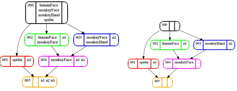
Figure 1: Concept lattice computed from the context in table 1. Each node is a concept, arrows represent superconcept relation, i.e. an arrow fromXtoY reads:Xis a superconcept ofY. Colors correspond to table 1, right. The number in the leftmost compartment is the concept number. Middle compartment contains the extent, rightmost compartment the intent. Left: fully labeled concepts, i.e. all members of extents and intents are listed in each concept node. Right: reduced labeling. An object/attribute is only listed in the extent/intent of the smallest/largest concept that contains it. Reduced labeling is very useful for drawing large concept lattices.

The lattice diagrams make the ordering relationship between the concepts graphically explicit: con-cept 3 contains all ”monkey-related” stimuli, concon-cept 2 encompasses all ”faces”. They have a com-mon child, concept 4, which is the ”com-monkeyFace” concept. The ”spider” concept (concept 1) is incomparable to any other concept except the top and the bottom of the lattice. Note that these re-lationships arise as a consequence of the (here hypothetical) response behavior of the neurons. We will show (section 5) that the response patterns of real neurons can lead to similarly interpretable structures.

From a decoding perspective, a fully labeled concept shows those stimuli that have activated at least the set of neurons in the intent. In contrast, the stimuli associated with a concept in reduced labeling will activate the set of neurons in the intent, but no others. The fully labeled concepts show stimuli encoded by activity of the active neurons of the concept without knowledge of the firing state of the other neurons. Reduced labels, on the other hand show those stimuli that elicited a responseonly

from the neurons in the intent.

3

Concept lattices of local, sparse and dense codes

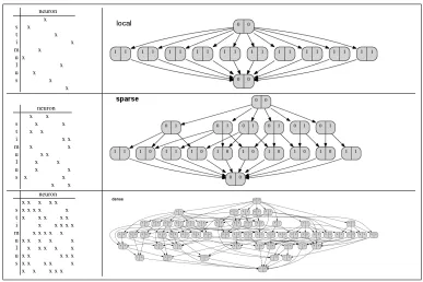
effects different levels of sparseness would have on a neural code, we generated random codes, i.e. each of 10 stimuli was associated with randomly drawn responses of 10 neurons, subject to the constraints that the code be perfectly decodable and that the sparseness of each codeword was equal to the sparseness of the code. Fig.2 shows the contexts (represented as cross-tables) and the concept lattices of a local code (activity ratio 0.1), a sparse code (activity ratio 0.2) and a dense code (activity ratio 0.5).

neuron x s x

t x

i x

m x

u x

l x

u x

s x

x

neuron x x

s x x

t x x

i x x

m x x

u x x

l x x

u x x

s x x

x x neuron x x x x x s x x x x x t x x x x x i x x x x x m x x x x x

u x x x x x l x x x x x u x x x x x s x x x x x

x x x x x

Figure 2: Contexts (represented as cross-tables) and concept lattices for a local, sparse and dense random neural code. Each context was built out of the responses of 10 (hypothetical) neurons to 10 stimuli. Each node represents a concept, the left(right) compartment contains the number of introduced stimuli(neurons). In a local code, the response patters to different stimuli have no overlapping activations, hence the lattice representing this code is an antichain with top and bottom element added. Each concept in the antichain introduces (at least) one stimulus and (at least) one neuron. In contrast, a dense code results in a lot of concepts which introduce neither a stimulus nor a neuron. The lattice of the dense code is also substantially longer than that of the sparse and local codes.

The most obvious differences between the lattices is the total number of concepts. A dense code, even for a small number of stimuli, will give rise to a lot of concepts, because the neuron sets repre-senting the stimuli are very probably going to have non-empty intersections. These intersections are potentially the intents of concepts which are larger than those concepts that introduce the stimuli. Hence, the latter are found towards the bottom of the lattice. This implies that they have large intents, which is of course a consequence of the density of the code. Determining these intents thus requires the observation of a large number of neurons, which is unappealing from a decoding perspective. The local code does not have this drawback, but is hampered by a small encoding capacity (maximal number of concepts with non-empty extents): the concept lattice in fig.2 is the largest one which can be constructed for a local code comprised of 10 binary neurons. Which of the above structures is most appropriate depends on the conceptual structure of environment to be encoded.

4

Building a formal context from responses of high-level visual neurons

nonlinearities and invariances which make it impossible to apply linear techniques, such as reverse correlation [18, 19, 20]. The concept lattice obtained by FCA might enable us to display and browse these invariances: if the response of a subset of cells indicates the presence of an invariant feature in a stimulus, then all stimuli having this feature should form the extent of a concept whose intent is given by the responding cells, much like the ”monkey” and ”face” concepts in the example in section 2.

4.1 Physiological data

The data were obtained through [21], where the experimental details can be found. Briefly, spike trains were obtained from neurons within the upper and lower banks of the superior temporal sulcus (STSa) via standard extracellular recording techniques [22] from an awake and behaving monkey (Macaca mulatta) performing a fixation task. This area contains cells which are responsive to faces. The recorded firing patters were turned into distinct samples, each of which contained the spikes from−300ms before to600ms after the stimulus onset with a temporal resolution of 1 ms. The stimulus set consisted of 1704 images, containing color and black and white views of human and monkey head and body, animals, fruits, natural outdoor scenes, abstract drawings and cartoons. Stimuli were presented for 55ms each without inter-stimulus gaps in random sequences. While this rapid serial visual presentation (RSVP) paradigm complicates the task of extracting stimulus-related information from the spiketrains, it has the advantage of allowing for the testing of a large number of stimuli. A given cell was tested on a subset of 600 or 1200 of these stimuli, each stimulus was presented between 1-15 times.

4.2 Bayesian thresholding

Before we can apply FCA, we need to extract a binary attribute from the raw spiketrains. While FCA can also deal with many-valued attributes, see [23, 9], we will employ binary thresholding as a starting point. Moreover, when time windows are limited (e.g. in the RSVP condition) it is usually impossible to extract more than 1 bit of stimulus identity-related information from a spiketrain per stimulus [24]. We do not suggest that real neurons have a binary activation function. We are merely concerned with finding a maximally informative response binarization, to allow for the construction of meaningful concepts. We do this by Bayesian thresholding, as detailed in appendix A. This procedure also avails us of a null hypothesisH0 =”the responses contain no information about the

stimuli”.

4.3 Cell selection

The experimental data consisted of recordings from 26 cells. To minimize the risk that the com-puted neural responses were a result of random fluctuations, we excluded a cell if 1.)H0was more

probable than10−6 _{or 2.) the posterior standard deviations of the counting window parameters}

were larger than20ms, indicating large uncertainties about the response timing. Cells which did not respond above the threshold included all cells excluded by the above criteria (except one). Fur-thermore, since not all cells were tested on all stimuli, we also had to select pairs of subsets of cells and stimuli such that all cells in a pair were tested on all stimuli. Incidentally, this selection can also be accomplished with FCA, by determining the concepts of a context withgJ m=”stimulusgwas tested on cellm” and selecting those with a large number of stimuli×number of cells. Two of these cell and stimulus subset pairs (”A”, containing 364 stimuli and 13 cells, and ”B”, containing 600 stimuli, 12 cells) were selected for further analysis.

5

Results

To analyze the neural code, the thresholded neural resposes were used to build stimulus-by-cell-response contexts. We performed FCA on these with COLIBRICONCEPTS1, created stimulus image montages and plotted the lattices2_{. The complete concept lattices were too large to display on a page.}

Graphs of lattices A and B with reduced labeling on the stimuli are included in the supplementary

1_{see http://code.google.com/p/colibri-concepts/} 2

A B

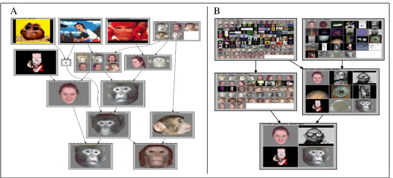
Figure 3: A: a subgraph of lattice A with reduced labeling on the stimuli, i.e. stimuli are only shown in their object concepts. The ∅ indicates that an extent is the intersection of its superconcepts’ extents, i.e. no new stimuli were introduced by this concept. All cells forming this part of the concept lattice were responsive to faces. B: a subgraph of lattice B, fully labeled. The concepts on the right side are not exclusively ”face” concepts, but most members of their extents have something ”roundish” about them.

material (fileslatticeA neuroFCA.pdfandlatticeB neuroFCA.pdf). In these graphs, the top of the frame around each concept image contains the concept number and the list of cells in the intent.

Fig.3, A shows a subgraph from lattice A, which exclusively contained ”face” concepts. This subgraph, with full labeling, is also a part of the supplementary material (file

faceSubgraphLatticeA neuroFCA.pdf). The top concepts introduce human and cartoon

faces, i.e. their extents are consist of general ”face” images, while their intents are small (3 cells). In contrast, the lower concepts introduce mostly single monkey faces, with the bottom concepts having an intent of 7 cells. We may interpret this as an indication that the neural code has a higher ”resolution” for faces of conspecifics than for faces in general, i.e. other monkeys are represented in greater detail in a monkey’s brain than humans or cartoons. This feature can be observed in most lattices we generated.

Fig.3, B shows a subgraph from lattice B with full labeling. The concepts in the left half of the graph are face concepts, whereas the extents of the concepts in the right half also contain a number of non-face stimuli. Most of the latter have something ”roundish” about them. The bottom concept, being subordinate to both the ”round” and the ”face” concepts, encompasses stimuli with both char-acteristics, which points towards a product-of-experts encoding [25]. This example also highlights another advantage of FCA over standard hierarchical analysis techniques, e.g. hierarchical cluster-ing: it does not impose a tree structure when the data do not support it (a shortcoming of the analysis in [26]).

6

Conclusion

We demonstrated the potential usefulness of FCA for the exploration and interpretation of neural codes. This technique is feasible even for high-level visual codes, where linear decoding methods [19, 20] fail, and it provides qualitative information about the structure of the code which goes beyond stimulus label decoding [4]. Clearly, this application of FCA is still in its infancy. It would be very interesting to repeat the analysis presented here on data obtained from simultaneous multi-cell recordings, to elucidate whether the conceptual structures derived by FCA are used for decoding by real brains. On a larger scale than single neurons, FCA could also be employed to study the relationships in fMRI data [27].

AcknowledgmentD. Endres was supported by MRC fellowship G0501319.

References

[1] A. P. Georgopoulos, A. B. Schwartz, and R. E. Kettner. Neuronal population coding of move-ment direction. Science, 233(4771):1416–1419, 1986.

[2] P F¨oldi´ak. The ’Ideal Homunculus’: Decoding neural population responses by Bayesian infer-ence. Perception, 22 suppl:43, 1993.

[3] MW Oram, P F¨oldi´ak, DI Perrett, and F Sengpiel. The ’Ideal Homunculus’: decoding neural population signals. Trends In Neurosciences, 21:259–265, June 1998.

[4] R. Q. Quiroga, L. Reddy, C. Koch, and I. Fried. Decoding Visual Inputs From Multiple Neu-rons in the Human Temporal Lobe. J Neurophysiol, 98(4):1997–2007, 2007.

[5] OR Duda, PE Hart, and DG Stork. Pattern classification. John Wiley & Sons, New York, Chichester, 2001.

[6] T. M. Cover and J. A. Thomas. Elements of Information Theory. John Wiley & Sons, New York, 1991.

[7] P F¨oldi´ak. Sparse neural representation for semantic indexing. In XIII Conference of the European Society of Cognitive Psychology (ESCOP-2003), 2003. http://www.st-andrews.ac.uk/∼pf2/escopill2.pdf.

[8] R. Wille. Restructuring lattice theory: an approach based on hierarchies of concepts. In I. Rival, editor,Ordered sets, pages 445–470. Reidel, Dordrecht-Boston, 1982.

[9] Bernhard Ganter and Rudolf Wille. Formal Concept Analysis: Mathematical foundations. Springer, 1999.

[10] B. Ganter, G. Stumme, and R. Wille, editors. Formal Concept Analysis, Foundations and Applications, volume 3626 ofLecture Notes in Computer Science. Springer, 2005.

[11] U. Priss. Formal concept analysis in information science. Annual Review of Information Science and Technology, 40:521–543, 2006.

[12] P F¨oldi´ak. Sparse coding in the primate cortex. In Michael A Arbib, editor,The Handbook of Brain Theory and Neural Networks, pages 1064–1068. MIT Press, second edition, 2002.

[13] P F¨oldi´ak and D Endres. Sparse coding. Scholarpedia, 3(1):2984, 2008. http://www.scholarpedia.org/article/Sparse coding.

[14] P F¨oldi´ak. Forming sparse representations by local anti-Hebbian learning. Biological Cyber-netics, 64:165–170, 1990.

[15] B. A Olshausen, D. J Field, and A Pelah. Sparse coding with an overcomplete basis set: a strategy employed by V1. Vision Res., 37(23):3311–3325, 1997.

[16] Eero P Simoncelli and Bruno A Olshausen. Natural image statistics and neural representation.

Annual Review of Neuroscience, 24:1193–1216, 2001.

[17] ET Rolls and A Treves. The relative advantages of sparse versus distributed encoding for neuronal networks in the brain. Network, 1:407–421, 1990.

[18] P Dayan and LF Abbott.Theoretical Neuroscience. MIT Press, London, Cambridge, 2001.

[20] D. L. Ringach. Spatial structure and symmetry of simple-cell receptive fields in macaque primary visual cortex. Journal of Neurophysiology, 88:455–463, 2002.

[21] P F¨oldi´ak, D Xiao, C Keysers, R Edwards, and DI Perrett. Rapid serial visual presentation for the determination of neural selectivity in area STSa. Progress in Brain Research, pages 107–116, 2004.

[22] M. W. Oram and D. I. Perrett. Time course of neural responses discriminating different views of the face and head. Journal of Neurophysiology, 68(1):70–84, 1992.

[23] R. Wille and F. Lehmann. A triadic approach to formal concept analysis. In G. Ellis, R. Levin-son, W. Rich, and J. F. Sowa, editors,Conceptual structures: applications, implementation and theory, pages 32–43. Springer, Berlin-Heidelberg-New York, 1995.

[24] D. Endres. Bayesian and Information-Theoretic Tools for Neuroscience. PhD thesis, School of Psychology, University of St. Andrews, U.K., 2006. http://hdl.handle.net/10023/162.

[25] GE Hinton. Products of experts. InNinth International Conference on Artificial Neural Net-works ICANN 99, number 470 in ICANN, 1999.

[26] R Kiani, H Esteky, K Mirpour, and K Tanaka. Object category structure in response pat-terns of neuronal population in monkey inferior temporal cortex. Journal of Neurophysiology, 97(6):4296–4309, April 2007.

[27] K. N. Kay, T. Naselaris, R. J. Prenger, and J. L. Gallant. Identifying natural images from human brain activity. Nature, 452:352–255, 2008. http://dx.doi.org/10.1038/nature06713.

[28] D. Endres and P. F¨oldi´ak. Exact Bayesian bin classification: a fast alternative to bayesian classification and its application to neural response analysis. Journal of Computational Neuro-science, 24(1):24–35, 2008. DOI: 10.1007/s10827-007-0039-5.

A

Method of Bayesian thresholding

A standard way of obtaining binary responses from neurons is thresholding the spike count within a certain time window. This is a relatively straightforward task, if the stimuli are presented well separated in time and a lot of trials per stimulus are available. Then latencies and response offsets are often clearly discernible and thus choosing the time window is not too difficult. However, under RSVP conditions with few trials per stimulus, response separation becomes more tricky, as the responses to subsequent stimuli will tend to follow each other without an intermediate return to baseline activity. Moreover, neural resposes tend to be rather noisy. We will therefore employ a simplified version of the generative Bayesian Bin classification algorithm (BBCa) [28], which was shown to perform well on RSVP data [24].

BBCa was designed for the purpose of inferring stimulus labelsgfrom a continuous-valued, scalar measurezof a neural response. The range ofzis divided into a number of contiguous bins. Within each bin, the observation model for thegis a Bernoulli scheme with a Dirichlet prior over its param-eters. It is shown in [28] that one can iterate/integrate over all possible bin boundary configurations efficiently, thus making exact Bayesian inference feasible. We make two simplifications to BBCa: 1)zis discrete, because we are counting spikes and 2) we use models with only 1 bin boundary in the range ofz. The bin membership of a given neural response can then serve as the binary attribute required for FCA, since BBCa weighs bin configurations by their classification (i.e. stimulus label decoding) performance. We proceed in a straight Bayesian fashion: since the bin membership is the only variable we are interested in, all other parameters (counting window size and position, class membership probabilities, bin boundaries) are marginalized. This minimizes the risk of spurious re-sults due to ”contrived” information (i.e. choices of parameters) made at some stage of the inference process. Afterwards, the probability that the response belongs to the upper bin is thresholded at a probability of 0.5. BBCa can also be used for model comparison. Running the algorithm with no bin boundaries in the range ofzeffectively yields the probability of the data given the ”null hypothesis”

H0: zdoes not contain any information aboutg. We can then compare it against the alternative