A User Selection Method in Advertising System

Int. J. Communications, Network and System Sciences, 2010, 3, 54-58

doi:10.4236/ijcns.2010.31007 Published Online January 2010 (http://www.SciRP.org/journal/ijcns/).

A User Selection Method in Advertising System

Shiyi XIONG, Zhiqing LIN, Bo XIAO

Pattern Recognition & Intelligent System Lab,Beijing University of Posts and Telecommunications, Beijing, China Email: [email protected], {linzq,xiaobo}@bupt.edu.cn

Received October 27,2009; revised November 28,2009; accepted December 30, 2009

Abstract

It’s important for mobile operators to recommend new services. Traditional method is sending advertising messages to all mobile users. But most of users who are not interested in these services treat the messages as Spam. This paper presents a method to find potential customers who are likely to accept the services. This method searchs the maximum frequent itemsets which indicate potential customers’ features from a large data set of users’ information, then find potential customers from those maximum frequent itemsets by using a bayesian network classifier. Experimental results demonstrate this method can select users with higher accuracy.

Keywords:User Selection, Maximum Frequent Itemsets, Bayesian Network

1. Introduction

Recent years, as the increasing number of mobile opera- tors and new services, the competition between operators becomes more and more furious. The key of the com- petition is to win more customers. How to introduce new services to proper customers becomes one of the major problems.

Now, advertising system mostly uses these technologies: collaborative filtering technology [1], content based re- commendation, knowledge based recommendation, effi- ciency based recommendation, association rules based recommendation [2], etc. These methods are usually used to select and recommend products to specified users. They analyse the user’s historical data and predict what products the user mostly need. For example, an online movie sys- tem uses one of above technologies to serve its user whose name is Mike. The system will analyse Mike’s history and recommend him some movies in which he may be interested. So we can say these methods solve the problem to select products for users.

The proplem we desire to solve in this paper is a little different. Here we have only one product, namely the new mobile service, and we want to know which users want to buy this service. Those users are potential customers, and we need to pick out them from a large number of users. The problem is to select users for one product. As a result, those traditional methods will not work well on this problem.

This paper presents a new method to select users. This method searchs the maximum frequent itemsets from a

large data set, then find potential customers from those maximum frequent itemsets by using a bayesian network classifier.

2. Analysis of Customer Features

Usually, mobile operators keep a large database of con- sumption data. This data includes the items that repre- sent customers’ features, such as the telephone fees of every month, function fees and information fees, etc. This data also shows whether a customer accepts the new service, those customers who accept new service can be seen as positive samples, and others can be seen as negative samples. As a result, the problem to select positive samples can be treated as a two-category classification problem.

Usually, two-category classification problem should have data with features shown in Figure 1(a). However, the mobile users’ data are quite different (shown in Figure 1(b). For example, some users who have the same features may belong to different categories. What’s more, number of negative samples is much larger than the number of positive sample. Because of this, routine classification methods such as naive bayesian classifier is hard to classfy such data.

3. Frequently Itemsets

3.1. Fomal Model of Frequently Itemsets

Let sampleXhas dimensions(Attributes) and the value may be continuous. Divide the value into several seg-

x2

x1 O

(a)

x

2

x

1

O

(b)

Figure 1. Feature distribution map. (a) Two-category classification; (b) Mobile users’ data.

ments and give each segment a unique serial code. Because each sample belongs to an segment, we can use the corresponding segment code to replace this sample. In this way, original samples X are mapped to the

segment codes Y :F X: Y.

Divide the original samples uses the following guidelines:

1) The number of positive samples in each segment is uniformly distributed.

2) Each Attributes should have the same number of segments.

Make each Attribute divided into k segments so that the segments code should not bigger than . If the value of a Attrubutes is a 0-1 type value, the number of segments code should be , not .

k

-1}

{0,1} {0,1,...,k

The Attribute segment i_j

m

is called item. The Attribute segment combination of attributes

is called itemsets. is length of the itemsets . If a sample’s attribute segments in dimensions are

, we call this sample satisfied the itemsets .

(

m mn

m

)

1 2 m {i ,i ,...,i }

I

1, ,...,2 m

i i i I

If an itemsets has positive sample number while has negative sample number b, is the

success rate of itemsets . Given a minimum support threshold

a )

b

/ (

i

f a a

I

. If a>, we call frequent itemsets. I

3.2. Frequent Close Itemset

Given be an itemsets with length m, add an item of attribute

1 2 { , ,..., }m

I i i i

m1 into , so

has the length

I I' { , ,..., , i i1 2 i im m1} 1

m . If and have the same number of

positive samples, then

I '

' I

I I

f  f . This can be proofed as

below:

Suppose both and have positive samples. has negative samples, while has . Since has one

more item 1

I I' a

b

I b I' ' I'

m

i _ ,we can getb≥b'. Thus

'

a a

abab

at is

,

th fI  fI', dan I'has a higher success ratio.

In case of fI  fI', ignore the itemsets , and keep . When

I I'

'

I I

f  f , is called frequent close itemsets(ab.

FCI). There are some typical algorithm to mine frequent close itemsets such as Apriori

I

[3] and FP2Tree [4]. As a part of the user selection method, samples in the FCI should be predicted using Bayesian network classifier. Given the number of attributes n and the number of segments k , then the number of itemsets is:

1

• ( 1)

N

i i N

N i

C M M



1

  



The number has an exponential growth, so it’s impossible to construct a Bayesian network classifier for all itemsets. A compromised way is colleting all of the samples to be one data set and construct a Bayesian network classifier based on this data set.

4. Bayesian Network Model for User

Selection

4.1. Bayesian Network Basics

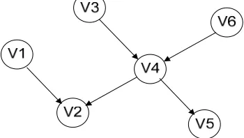
A Bayesian network is a graphical model that encodes relationships among variables of interest. A Bayesian network consists of a set of nodes and a set of directed edges between nodes [5], which shown in Figure 2. In general, a Bayesian network is expressed as sign

( , )

B G P , which consists of the following two parts [6].

S. Y. XIONG ET AL.

56

1) A directed acyclic graphGwith nodes. The nodes

of the graph represent random variables or events. The directed edges between nodes in the graph represent the causal relationships of the nodes. The important concept in Bayesian networks is the conditional independence between variables. For any variable , the parent vari- ables of is , the is independent of the variables set

n

i V

i

V pa V( )i

( )i

i V

A V , which is the set of the variables that

are not child variables of , so the probability of is calculated as:

(Vi) pa

i V

log

( | ) | | ( | )

2

N

MDL B D  B LL B D

where | |B is the number of parameters in the network.

The second term is the negation of the log likelihood of

B given : D

( ) 1

( | ) log( ) i

N

B u i

LL B D P







Bayesian network structure learning is NP problem, now typical method has K2 [8] developed by Cooper and Hers2kovits.

( | ( ),i i ( ))i ( |i ( ))i

p V A V pa V  p V pa V

5. Model of Selection Method

ciated with each node . The CPT is expressed as which pictures the mutual relationship of each node and its parent nodes. Nodes with no parent have a very simple probability table, giving the prior probability distribution of the node. Nodes with parents are much more complicated. These nodes have condi- tional probability tables, which give a probability distri- bution for every combination of states of the variable’s parents.

P

( |i ( ))i

P V pa V The method searchs the maximum frequent itemsets

from a large data set, then find potential customers from those maximum frequent itemsets by using a bayesian network classifier. In detail, we can get result by taking following steps:

1) All users share the same attributes. For each attribute, users have different values from each other. We get all sample’s values of each attribute from the data set, and divide these values into k segments using the method presented in Subsection 2.2.1.

The Bayesian network can represent all of the nodes’ joint probability due to the node relationship and the conditional probability table. Applying the conditional independence into the chain rule, we get the following expression:

2) Based on the data processing in step 1, set a minimum support number and mine all of the FCI.

3) Every FCI contain a certain number of samples, collect these samples and make them to be a new data set

.

D

1 2

1

( , ,... ) ( | ( ))

n

n i

i

p V V V p V pa V







4) Learn bayesian network from data set which is formed in step 3, using K2 algorithm.

D

5) For samples without knowing is positive or is negative, calculate its positive probability by bayesian network constructed in 4. Once we get the probability, we can get result by comparing it with given threshold.

4.2. Bayesian Network Structure Learning

Consider a finite set of discrete random variables where each variable may take on values from a finite set, denoted by . Formally, a Bayesian network for U is a pair

1 2 { , ,... }n

U  V V V

i V

( )i Val V

,

BG  , and defines a

unique joint probability distribution over U . The

problem of learning a Bayesian network can be informally stated as: Given a training set D

of instances of U, find a network 1 2

{ , ,... }u u un B that

best matches D. The common approach to this pro- blem is to introduce a scoring function that evaluates each network with respect to the training data, and then to search for the best network according to this function. The two main scoring functions commonly used to learn Bayesian networks are the Bayesian scoring function [8], and the function based on the principle of minimal description length (ab. MDL) [7]. We only introduce MDL scoring function. The MDL scoring function of a network B given a training data set D , written

( | )

MDL B D , is given by following expresion:

If a user is predicted to be positive, then the recom- mendation system will send the advertisement message to this user. On the other hand, user who are predicted to be negative will not receive advertisement messages.

6. Experiment

In experiments we try the new method as well as method based on naive bayesian claasifier so that we can com- pare the results between both methods.

6.1. Classify Using Naive Bayesian Classifier

1) Discretize the values and train naive bayesian classi- fier.

0.0975

0.0986

0.0974

0.096

0.094 0.095 0.096 0.097 0.098 0.099

5 10 20 30

Number of segments

Success rate

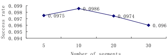
Figure 3. Success rate for different segments number.

0 0.05 0.1 0.15 0.2

10 20 30 40 50

Minimum support number counter

Succ

ess ra

te

Figure 4. Success rate for different Minimum support number.

Figure 5. Bayesian network learned by GENIE.

6.2. Steps of New Method

1) We divide the values of each attribute into k segments. While k is 10, 20, 30 respectivly, the results are shown in Figure 3. It shows that the best result occurs while k is 10.

2) Given a minimum support number  and search FCI, then compare the experimental results when  is 10, 20, 30, 40, 50 respectivly. The results are shown in Figure 4. It shows that we get the highest success rate while  is 50. We don’t consider a minimum support number larger than 50 because the coverage of potential customer will decrease too much, see the data in Table 2.

3) Learn bayesian network from D using a open source bayesian tool called GENIE (http://genie.sis.pitt.edu), which uses K2 algorithm to learn Bayesian network structure. We get a Bayesian network shown in Figure 5, where GPRS_ FLOW, MMS_FEE, etc are names of attributes. YND-SUCCESS is the target attribute to be predicted.

4) Last step is predicting by Bayesian network classi-fier. Since the number of negative samples is much more large than number of positive samples, we set the thresh-old to be 0.1. That means if a sample has a probability to be positive sample larger than 0.1, then it is determined to be positive.

6.3. Experimental Results

In this experiment, we use a data set from a mobile ser-vice provider. We divide the users into two parts. One part with the user number of 12264 is training data set. The other part with 12263 users including 577 positive users is test data set.

For traditional method which sends advertising mes-sage to all users. It sends 12264 advertisements and gets 577 customers, the success rate is 4.7%. It sends adver-tisement to 100% of the users, and gets 100% of the po-tential customers.

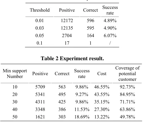
For method based on naïve Bayesian classifier whose results shown in Table 1, the results are almost the same as the results of traditional method. Obviously, naïve Bayesian classifier does not work well with mobile user’s data set.

For new method, the results are shown in Table 2. Take mininum support number 50 for example, it sends 1621 advertisements and gets 303 customers, the success rate is 18.69%. It sends advertisement to 13.22% of all users, and gets 49.78% of the potential customers.

S. Y. XIONG ET AL.

58

Table 1. Results of naïve Bayesian classifier.

Success Threshold Positive Correct _rate

0.01 12172 596 4.89% 0.03 12135 595 4.90% 0.05 2704 164 6.07%

0.1 17 1 /

ble 2 Experiment sult.

in support Number Pos

Coverage of potential

Ta re

M _{itive Correct} Success

rate Cost _customer

10 5709 563 9.86% 46.55% 92.73% 20 5341 495 9.27% 43.55% 84.95% 30 4311 425 9.86% 35.15% 71.71% 40 3348 386 11.53% 27.30% 63.86% 50 1621 303 18.69% 13.22% 49.78%

rate 5%, i ati h su te

f traditional method and of naïve Bayesian classifi

sions

em becomes more and more im tan service providers now. User selection is one of th

w

8. Acknowledgement

Th work was supported by the national High-tech

. References

] E. Rich, “User modeling via stereotypes [D],” Cognitive

d P. Smyth,

ms for mining

ing frequent

Bayesian networks,”

and reasoning with

probabil-ldszmidt, “Bayesian

per and E. Herskovits, “A Bayesian method for

9.8 s dram cally igher than the ccess ra

“Ad

o er. It association rules in large databases [R],” IBM Almaden

Research Center, Tech Rep: RJ9839, 1994. [4] J. W. Han, J. Pei, Y. W. Yin, et al., “Min

also saves advertising cost and cuts down Spam re-markably.

7. Conclu

Recomendation syst por-

e Springer, New York, 1996.

[6] M. desJarins, “Representing

t to

difficulty problems. This paper presents a method to select users, the method searchs the maximum frequent itemsets from a large data set, then find potential cus- tomers from those maximum frequent itemsets by using a bayesian network classifier. The success rate is im-proved dramatically after using the method. This method also cuts down advertisement cost for mobile operators and avoids making large number of Spam messages.

There are a lot of data sets which have similar features

ith mobile user’s data set, so this method can be used in many similar advertising recommendation systems. It has a good universality.

is

Research and Development Plan of China under grant No.2007AA01Z417 and the 111 Project of China under grant No. B08004.

9

[1

Science, Vol. 3, No. 4, pp. 329–354, 1979. [2] U. M. Fayyad, G. Piatecsky-Shapiro, an

vances in knowledge discovery and data mining [M],” California, AAAI/MIT Press, 1996.

[3] R. Agrawal and M. Srikant, “Fast algorith

patterns without candidate generation: A frequent-pattern tree approach [J],” Data Mining and Knowledge Discov-ery, Vol. 8, No. 1, pp. 53–87, 2004.

[5] F. V. Jensen, “An introduction to

istic knowledge: A Bayesian approach,” Uncertainty in Artificial Intelligence, pp. 227–234.

[7] N. Friedman, D. Geiger, and M. Go

network classifiers,” Machine Learning, pp.131–163, 1997.

[8] G. Coo