A relative evaluation of multi-class image classification by support vector machines
Giles M. Foody and Ajay Mathur
IEEE Transactions on Geoscience and Remote Sensing, 42, 1335-1343 (2004)
The manuscript of the above article revised after peer review and submitted to the journal for publication, follows. Please note that small changes may have been made after submission and the definitive version is that subsequently published as:
A relative evaluation of multi-class image classification by support vector machines
Giles M. Foody and Ajay Mathur School of Geography
University of Southampton Highfield
Southampton SO17 1BJ UK
ABSTRACT
Support vector machines (SVM) have considerable potential as classifiers of remotely sensed data. A constraint on their application in remote sensing has been their binary nature,
I. INTRODUCTION
Land cover is a critical variable that links many parts of the human and physical
environments. Accurate and up-to-date information on land cover is required for a plethora of applications, including land resource planning, studies of environmental change and
biodiversity conservation. Realistically, the only feasible source of information on land cover over large areas and which allows data to be acquired in a regularly repeatable manner is remote sensing. Despite the great potential of remote sensing as source of information on land cover and the long history of research into the extraction of land cover information from remotely sensed imagery, many problems have been encountered and the accuracy of land cover maps derived from remotely sensed imagery has often been viewed as too low for operational users [1, 2]. Many factors may be responsible for the problems encountered. These include the nature of the classes (e.g. discrete or continuous), the properties of the remote sensor (e.g. its spatial and spectral resolutions), the nature of the land cover mosaic (e.g. degree of fragmentation) and the methods used to extract the land cover information from the imagery (e.g. classification methods). These various problems have driven research into a diverse range of issues focused on topics such as sensor design, class definition protocols and image analysis techniques. Here, attention is focused on some aspects associated with the latter issue.
Many of the problems in mapping land cover noted in the literature relate to the methods used to extract the land cover information from the imagery. This has driven a considerable
likelihood classification. The problems associated with satisfying the assumptions that underlie such classifications has driven research into non-parametric alternatives including techniques such as evidential reasoning [3, 4] and more recently neural networks [5-7] and decision trees [8-10]. Although the accuracy with which land cover may be classified by these techniques has often been found to be higher than that derived from the conventional
statistical classifiers [e.g. 11-14] there is still considerable scope for further increases in accuracy to be obtained and a strong desire to maximise the degree of land cover information extraction from remotely sensed data. Thus, research into new methods of classification has continued and support vector machines (SVM) have recently attracted the attention of the remote sensing community [15-17]. Key attractions of the SVM based approach to
classification are that it seeks to fit an optimal hyperplane between classes and may require only a small training sample [15, 18, 19].
Although the potential of support vector machines is evident and early studies have demonstrated considerable success in using them to map land cover accurately there are problems in their usage. One of the main concerns is that SVMs were originally defined as binary classifiers and their use for multi-class classifications is more problematic, with strategies that reduce the multi-class problem to a set of binary problems typically adopted. Because multi-class problems are commonly encountered, researchers have sought to extend the basic binary SVM approach to form a multi-class classifier [20-24]. Recently, an
approach for a ‗one-shot‘ multi-class SVM classification has been reported [25] that has great potential for application in remote sensing. This multi-class SVM is particularly attractive for classification since key parameters (C and γ, defined below) need only be defined once rather than for each binary analysis and, as fewer support vectors may be required, it may be
multi-class SVM approach to land cover mapping relative to a suite of other popular
classifiers. In particular this evaluation focuses on the accuracy with which a data set may be classified using differentially sized training sets. The paper is structured such that we first introduce the fundamentals of SVM classification in the next section. In section III the remotely sensed data sets and classification methods used are outlined. In section IV the means by which classification accuracy was assessed and, critically, compared in a statistically rigorous fashion is discussed before presenting the results in section V and concluding in section VI.
II. SVMs
SVMs are very attractive for the classification of remotely sensed data. This approach seeks to find the optimal separating hyperplane between classes by focusing on the training cases that lie at the edge of the class distributions, the support vectors, with the other training cases effectively discarded [18, 19, 26]. Thus not only is an optimal hyperplane fitted but also the approach may be expected to yield high accuracy with small training sets, which given the costs of training data acquisition in remote sensing could be a very advantageous feature. The basis of the SVM approach to classification is, therefore, the notion that only the training samples that lie on the class boundaries are necessary for discrimination.
between the two classes, with all cases of a class located to one side of the separating hyperplane which is itself located such that the distance to the closest training data points in both of the classes is as large as possible.
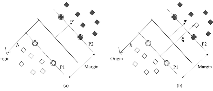
A hyperplane can be defined by the equation w.x+ b = 0, where x is a point lying on the
hyperplane, w is normal to the hyperplane, b is the bias and
w b
is the perpendicular distance
from the hyperplane to the origin (Figure 1), with w the Euclidean norm of w. For the linearly separable case, a separating hyperplane can be defined for the two classes as:w.xi b1(for yi 1) and w.xib1(for yi 1). The two equations can be combined as:
0 1 )
( b
yi w.xi (1)
The training data points on these two hyperplanes are called as support vectors and are central to the establishment of the optimal separating hyperplane. The support vectors of the two classes lie on two hyperplanes, which are parallel to the optimal hyperplane and are defined
by w.xi b1. The margin between these planes is
w
2
. The maximization of this margin
leads to the following constrained optimization problem,
min }
2 1
{ w 2 (2)
Commonly, the classes are not linearly separable and the constraints of equation 1 cannot be satisfied. To deal with such cases using only linear separating boundaries, a new set of variables, sometimes referred to as slack variables,{i}ir1, that indicate the distance the case is from the optimal hyperplane (Figure 1) and so the amount of violation of the constraints may be introduced. The constraint then becomes,
i i b
y(w.x )1 (3)
The above constraint, in case of outliers, can always be met by making i very large, so, a
penalty term,
r i i C 1
is added to penalize solutions for which i are very large. The constant
C controls the magnitude of the penalty associated with training samples that lie on the wrong side of the decision boundary. With a low value of C, an inappropriately large a fraction of support vectors may be derived while with a large value of C there is a danger of the SVM over-fitting to the training data and so having low generalization ability. In practice, however, a considerable degree of robustness of SVM based classification to variation in its parameters has been noted [19]. With the addition of the penalty term, the optimization problem
becomes, ] 2 min[ 1 2
r i i C w (4)[19]. If the classes overlap considerably in feature space, then
r i i C 1 can be very large and
the hyperplane may not generalize well.
The basic approach outlined above may be extended to allow for non-linear decision surfaces. For example, the input data may be mapped into a high dimensional space through some non-linear mapping which has the effect of spreading the distribution of the data points in a way that facilitates the fitting of a linear hyperplane. Specifically, the training data may be projected into a high dimensional, Hilbert, space H, through a mapping function φ, or
H Rq
φ: . An input data point x can be represented as φ(x) in the high dimensional
space H. The expensive computation of (φ(x),φ(xi))in a high dimensional space is reduced by using a positive definite kernel such that:
) , ( )) ( ), (
(φ x φ xi k x xi (5)
leading to decision functions of the form;
) ) , ( sgn( ) ( 1 b k y x f i r i i i
x x (6)
2 ) (
) ,
( i
e
k x xi x x (7)
where γ is the parameter controlling the width of the Gaussian kernel. The accuracy of classification by a SVM is dependent on the magnitude of the parameters C and γ. With a
large value of γ and/or C, there is a tendency for the SVM to over-fit to the training data, yielding a classifier that may generalize poorly. In such circumstances, it may be possible to classify the training data accurately but the accuracy with which an independent testing set is classified may be small. Consequently, the magnitude of C and γ must be determined carefully. In practice, a large generalization ability may be obtained by setting γ appropriately given a defined value for C. If ground data are plentiful, it may be possible to use a cross-validation approach or a cross-validation set, distinct from both the training and testing sets, to help select appropriate values for the parameters or to predict the generalization ability directly from the training set [19].
Unfortunately, however, SVMs were originally designed for binary classification yet most remote sensing applications involve multiple classes. For the benefit of the SVM approach to be realised in remote sensing, therefore, some means of extending the SVM approach to classification to multi-class situations is required.
after solving equation 4, for a case xithere are n decision functions, where n is the number of classes,
i i
i b
) ( )
(w φ x , where i=1,….n
The data xi then belongs to the class, for which the above decision function has the largest value. That is,
class of xi = argmax i=1, …., n((wi)φ(xi)bi) (8)
This approach has been used to map land cover from remotely sensed data [e.g. 15]. As well as requiring n analyses to be undertaken this approach may suffer from error caused by markedly imbalanced training sets.
The second method of reducing a multi-class problem to a series of binary ones to enable the application of the basic SVM model for multi-class classification is the ‗one against one‘ approach. In this, a series of classifiers are applied to each pair of classes, with the most commonly computed class label kept for each pixel. The application of this method requires
Multi-class classifications of remotely sensed data by SVM have to-date been based mainly on the above approaches [e.g. 15, 17, 18, 30]. While both strategies to reducing the multi-class problem to a set of binary multi-classifications enable the basic SVM to be employed, a more appropriate approach may be to consider all classes at one time, yielding a multi-class SVM [25]. One means to achieve this, which is similar in basis to the ‗one-against-all‘ approach, is by solving a single optimisation problem. With this, n two class rules where the mth function
b m ) (x φ
w separates the training data vectors of class m from that of others are constructed. Hence, there are n decision functions or hyperplanes but all are obtained by solving one problem,
i y m m i l i m n m m bw C ,
1 1 , , 2 1 min
w w , (9)
under the constraints,
m i m i m y i
yi ( )bi ( )b 2, x φ w x φ w , i m
i, 0,i1,...,l,m{1,....n}\ y
where i=1,…,l are the training data vectors. The decision function is then,
argmax m=1,…n (wmφ(xi)bm) (10)
In reducing the classification to a single optimization problem this approach may also require fewer support vectors than a multi-class classification based on the combined use of many binary SVMs [25]. Additionally, with the multi-class SVM approach the values for the parameters C and γ need only to be defined once.
III. DATA AND METHODS OF CLASSIFICATION
Imagery acquired by an airborne thematic mapper (ATM) was used. These data were acquired by a Daedalus 1268 ATM in July 1986 over an agricultural region adjacent to the village of Feltwell in Eastern England. The data were acquired in 11 spectral wavebands with a spatial resolution of approximately 5 m. Near the time of the ATM data acquisition a crop map for the test site was constructed by conventional field survey methods. This map identified the single crop type planted in the fields, which were very large in comparison to the spatial resolution of the imagery.
Most of the test site had been planted to wheat, sugar beet, carrots, barley, grass and potatoes. Focusing on just these six classes, a stratified random sample of 100 pixels per-class was derived for each class and available for use in training the classification analyses. Training sets comprising a sample of between 15 and all 100 pixels per-class were constructed to allow the effect of training set size on classification accuracy to be evaluated. Since the results of a classification may be highly dependent on the specific sample of pixels selected, for each size of training set, except that using all 100 pixels available for each class, five independent samples were derived from the available training data. For each training set size, each of the five training sets was used to train a classification and, to avoid extreme results, the main focus here is on the classification with the median accuracy. Accuracy was assessed using a further, independent, random sample of 320 pixels that was acquired for use as a testing set. This testing set was used in the evaluation of the accuracy of all the classification analyses undertaken.
of the analyses to ensure that the sampled pixels were located within the relatively homogeneous cover of the crop planted in the large fields.
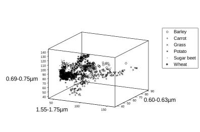
From previous research with this data set it was apparent that the data in all 11 wavebands were not required [31]. Here, the three wavebands identified as providing the greatest level of inter-class separability were selected for the analyses. These were the 0.60-0.63, 0.69-0.75 and 1.55-1.75 μm wavebands and the location of the classes in the feature space they define is shown in Figure 2.
The multi-class SVM approach with a RBF kernel and C=1 was used to classify the data. Since the accuracy of the classification may vary with the γ parameter, the relationship between accuracy and γ, sampled over the range 0.005 to 1.0, was defined for each analysis. For each of the training sets used, the results for the most accurate classification of the testing set were derived and the median value selected. Some implications of this approach for the relative evaluation of the SVM against more conventional classifiers is discussed below after first outlining the other classifiers used in this study.
In addition to the multi-class SVM approach to classification outlined above, three other classifiers were used. These were a discriminant analysis, decision tree and feedforward neural network.
assessed. Furthermore, as a basic statistical classifier, a major concern in the training stage of the classification is to derive a representative description of each class, specifically of its mean and variance. Consequently, it is typically recommended that the training set comprise, as a minimum, a sample of typically 10-30 pixels per-class per-waveband used [32]. Such a sample size is, on the assumption that the data are normally distributed, deemed to provide an appropriate summary of the data‘s distribution from which a representative estimate of the mean and variance may be derived.
The decision tree algorithm used the gain ratio to split nodes and the pessimistic error rate in tree pruning [33]. Again the size of the training set can influence classification accuracy and other studies have shown that the accuracy of decision tree classification increases with training set size [14].
The neural network used was a basic multi-layer perceptron. The network‘s architecture and algorithm parameters were defined from an evaluation of several hundreds of candidate networks. Previous studies have shown that the training set, notably in terms of its size and composition can have a marked impact on the accuracy of classification by a neural network [34-36]. Moreover, it is apparent that the individual training cases vary in importance, with those lying close to the class borders most informative and helpful in determining the location of the classification hyperplanes [37].
rather than individually. This may be valuable as ensemble based approaches can yield accurate image classifications [38-41].
For fair comparison of the classifications it is important to note some important implications associated with the methodology adopted. Although the generalization ability of the SVM may be relatively robust to variation in the parameter settings used [19], the method used to define γ in the SVM classification will ensure a high accuracy was derived. To facilitate fair comparison an approach that helps to identify appropriate parameter settings was adopted, if appropriate, for the other classifiers. Thus, for example, the parameters of the neural network classifiers were also defined in a manner that would help ensure high accuracy. Specifically, the learning algorithm and architecture of the neural networks used were defined from trials of hundreds of candidate networks using a software package that sought to define an optimal network in terms of the accuracy with which the testing set is classified. Thus, both the SVM and neural network classifiers have been defined in a manner that helps ensure a high
cross-validation and validation set based approaches to the selection of SVM and, where appropriate, neural network parameters are presented to facilitate fair comparison of these classifiers. For brevity, and since these analyses are intended to show that the methodology adopted did not lead to significant bias in the results, these analyses focus on just a single training set size. Two approaches to aid the parameterization of the classifiers were evaluated. First, five-fold cross validation (using a random sample of one fifth of the training set for validation purposes) to define γ in the SVM was evaluated for the situation in which 75 training cases were available. Second, an independent validation set of 25 cases was used together with 75 training cases to select appropriate parameters for both the SVM and neural network classifiers. As with the main analyses, these analyses were repeated five times and the median accuracy reported.
IV. ACCURACY ASSESSMENT AND COMPARISON
Fundamental to this work is the comparison of classification accuracy statements. The evaluation and comparison of classifications is plagued with problems [2]. Classification accuracy is commonly expressed using a metric computed from the error or confusion matrix using the testing set and estimates for different classifications compared to indicate the significance of differences in the classification outputs. One approach that has been used commonly in remote sensing is to express accuracy in terms of the kappa coefficient of agreement and use a Z test to evaluate the significance of differences in classification accuracy [e.g. 42]. However, there are many problems with this type of approach. For example, the kappa coefficient may be an inappropriate metric [43, 44] and the comparative method used typically assumes independent samples which is often, and here, not the
accuracy in land cover studies, was calculated for each classification and used to represent classification accuracy. The confusion matrices are, however, presented for the analyses based on the largest training set size to indicate the pattern of class allocations and, if appropriate, enable other metrics of accuracy to be derived if desired.
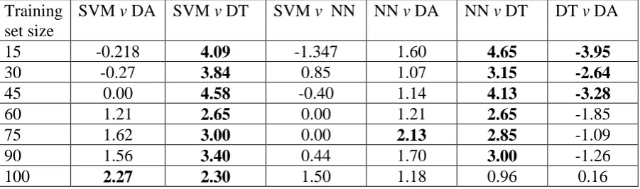
The comparison of classification accuracy statements should be undertaken in a statistically rigorous fashion. Here, the statistical significance of differences in the accuracy of
classifications derived using different methods was assessed using a McNemar test, without correction for continuity, for related samples. This is a non-parametric test that may be applied to confusion matrices that are 2x2 in dimension, which is the situation in classification comparison in which the two classes represent the instances when the classifications compared agree or disagree [45]. This test is based upon the standardised normal test statistic,
21 12
21 12
f f
f f
(11)
in which f12 and f21 represent the off-diagonal entries in the matrix. The analysis may
sometimes be based on a chi-square (2) distribution; the square of Z follows a chi-squared distribution with 1 degree of freedom.
V. RESULTS AND DISCUSSION
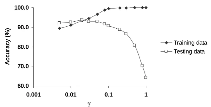
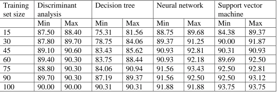
analysis (p<0.05). The value of the γ parameter had a marked impact on classification accuracy (Figure 4). In the SVM classifications reported, the γ parameter ranged from 0.005 to 0.08. The number of support vectors used ranged from 74 to 331.
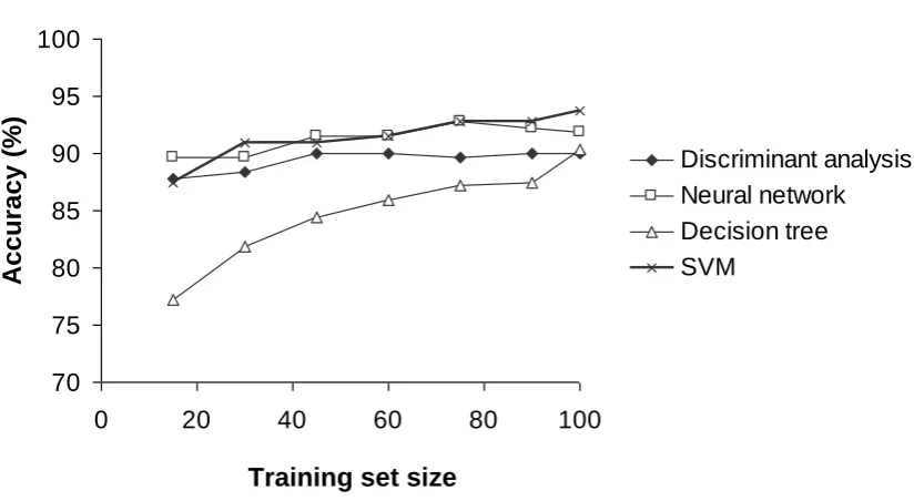
With all four classification methods it was apparent that classification accuracy was positively related to training set size (Figure 5). For the SVM based classifications, the difference in accuracy between the classifications trained on the largest and smallest training sets was 6.25%. Classification by the decision tree algorithm appeared to be most sensitive to training set size, with the accuracy increasing from 77.18% to 90.31% as the training set increased from containing 15 to 100 cases of each class. For all classifiers, except the neural network, the difference in the accuracy of the classifications derived with the use of the largest and smallest training sets was statistically significant (p<0.05). At each training set size, the SVM was also relatively accurate and often the most accurate classifier, with accuracies often statistically different from those derived from the other classifiers (Table 1).
classification may be based on the information provided by a small number of training sites, forming the support vectors, a large training sample may still be required to ensure that appropriate support vectors are available.
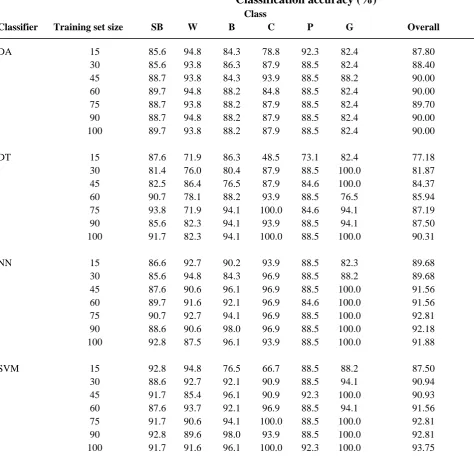
Although the four classifiers were able to classify the data very accurately, each >90% accurate for the analyses based on the largest training set size, there were some important differences. It was apparent, for example, that the classifiers varied in their ability to distinguish between specific classes and the accuracy with which individual classes were classified differed markedly (Table 3). Since the four classifiers operated in very different ways, they may be viewed as complimentary sources of information rather than competing options. This may make them useful candidates for use in a consensual or ensemble based approach to image classification. For example, 8 cases of sugarbeet in the testing set were misclassified by the SVM (Figure 3). Of these, 2 were misclassified by all four classifiers but a correct allocation made by at least one of the other classifiers for the other 6 cases.
Moreover, for 5 of these cases the correct allocation was made by the decision tree
classification. Similarly, there were 8 cases of wheat in the testing set that were misclassified by the SVM. Half of these cases were correctly allocated by the discriminant analysis.
Finally, to ensure mainly that the results of the SVM classifications had not been
optimistically biased by the methodology adopted in their parameterization, classifications using cross-validation and validation set based approaches to parameterization were
Although the results are data-specific and sensitive to how the classifiers were parameterised they do indicate the value of multi-class SVM classification. The SVM classifications were generally more accurate than comparator analyses and, with the analyses constrained to a single optimization problem, rapid computationally. As a guide to processing time the most rapid classifications were by the discriminant analysis but classification by the SVM approach was faster than both the decision tree and neural network classifications. Classification
accuracy was, however, a function of training set size and the potential of using small training sets in SVM based classification will require a means of intelligent training data acquisition.
VI. CONCLUSIONS
SVMs have considerable potential for the classification of remotely sensed data. To-date the use of SVMs for multi-class classification has been based mainly on the use of multiple binary analyses. It has been demonstrated here that a single multi-class SVM classification may be undertaken and used to derive very accurate classifications. In general, the SVM classifications were more accurate than comparable classifications derived with the use of the other classification techniques. The accuracy of the classifications produced from all of the classifiers was positively related to training set size, with the accuracy of the classifications derived from three of the classifiers increasing significantly as the training set size increased from 15 to 100 cases per-class. Although a SVM classification is effectively based on a small number of training sites a large training sample may still, therefore, be required to ensure that appropriate training data are included. Finally, the results show that the classifiers differ in the allocations made for individual cases and, in order to utilise their different merits, may be attractive as parts of a consensual or ensemble based approach to classification.
We are grateful to the Commission of European Community for the data sets which were acquired as part of the European AgriSAR campaign and the provision to AM of a Commonwealth Scholarship and leave of absence from Punjab Remote Sensing Centre, Ludhiana, India to undertake postgraduate research at Southampton University. The neural networks used were constructed with the NCS Neural Desk package. The decision tree was based on CTree algorithm developed by Angshuman Saha. The support vector machines were constructed with BSVM (version 2.01) software developed by Chih-Wei Hsu and Chih-Jen Lin, National Taiwan University, Taipei. We are also grateful to the three referees for their constructive comments on the original manuscript.
REFERENCES
[1] Wilkinson, G. G., ―Classification algorithms – where next?,‖ In E Binaghi, P. A. Brivio and A. Rampini (Eds) Soft Computing in Remote Sensing Data Analysis, Singapore: World Scientific, pp. 93-99, 1996.
[2] Foody, G., M., ―Status of land cover classification accuracy assessment,‖ Remote Sens. Environ., vol. 80, pp. 185-201, 2002.
[3] Peddle, D. R. and Franklin, S. E., ―Multisource evidential classification of surface cover and frozen ground,‖ Int. J. Remote Sens., vol 13, pp. 3375-3380, 1992.
[5] Benediktsson, J. A., Swain, P. H. and Ersoy, O. K., ―Neural network approaches versus statistical-methods in classification of multisource remote-sensing data,‖ IEEE Trans. Geosci. Remote Sensing, vol. 28, pp. 540-552, 1990.
[6] Kanellopoulos, I. and Wilkinson, G. G., ―Strategies and best practice for neural network image classification,‖ Int. J. Remote Sens., vol. 18, pp. 711-725, 1997.
[7] Liu, C. M., Zhang, L. J., Davis, C. J., Solomon, D. S., Brann, T. B. and Caldwell, L. E., ―Comparison of neural networks and statistical methods in classification of ecological habitats using FIA data,‖ Forest Science, vol. 49, pp. 619-631, 2003.
[8] Goel, P. K., Prasher, S. O., Patel, R. M., Landry, J. A., Bonnell, R. B. and Viau, A. A., ―Classification of hyperspectral data by decision trees and artificial neural networks to identify weed stress and nitrogen status of corn,‖ Computers and Electronics in Agriculture, vol. 39, pp. 67-93, 2003.
[9] McIver, D. K. and Friedl, M. A., ―Using prior probabilities in decision-tree classification of remotely sensed data,‖ Remote Sens. Environ., vol. 81, pp. 253-261, 2002.
[11] Peddle, D. R., Foody, G. M., Zhang, A., Franklin, S. E. and LeDrew, E. F., ―Multisource image classification II: an empirical comparison of evidential reasoning and neural network approaches,‖ Can. J. Remote Sens., vol. 20, 396-407, 1994.
[12] Rogan, J., Franklin, J. and Roberts, D. A., ―A comparison of methods for monitoring multitemporal vegetation change using Thematic Mapper imagery‖, Remote Sens. Environ, vol. 80, pp. 143-156, 2002.
[13] Li, T. S., Chen, C. Y. and Su, C. T., ―Comparison of neural and statistical algorithms for supervised classification of multi-dimensional data,‖ International Journal of Industrial Engineering-Theory Applications and Practice, vol. 10, pp. 73-81, 2003.
[14] Pal, M. and Mather, P. M., ―An assessment of the effectiveness of decision tree methods for land cover classification,‖ Remote Sens. Environ., vol. 86, pp. 554-565, 2003.
[15] Huang, C., Davis, L. S. and Townshend, J. R. G., An assessment of support vector machines for land cover classification, Int. J. Remote Sens., vol. 23, pp. 725-749, 2002.
[16] Brown, M., Gunn, S. R. and Lewis, H. G., ―Support vector machines for optimal classification and spectral unmixing,‖ Ecol. Mod., vol. 120, pp. 167-179, 1999.
[18] Mercier, G. and Lennon, M., 2003, Support vector machines for hyperspectral image classification with spectral-based kernels, Proceedings IEEE International Geoscience and Remote Sensing Symposium, 21-25 July 2003, Toulouse, IEEE Piscataway, CD-ROM, 2003.
[19] Belousov, A. I., Verzakov, S. A. and von Frese, J., ―A flexible classification approach with optimal generalisation performance: support vector machines,‖ Chemometrics and Intelligent Laboratory Systems, vol 64, pp. 15-25, 2002.
[20] Perez-Cruz, F. and Artes-Rodriguez, A., ―Puncturing multi-class support vector machines,‖ Lecture Notes in Computer Science, vol. 2415, pp. 751-756, 2002.
[21] Angulo, C., Parra, X. and Catala, A., ―K-SVCR. A support vector machine for multi-class multi-classification,‖ Neurocomputing, vol. 55, pp. 57-77, 2003.
[22] Lee, Y. and Lee, C. K., ―Classification of multiple cancer types by tip multicategory support vector machines using gene expression data,‖ Bioinformatics, vol. 19, pp. 1132-1139, 2003.
[24] Zhu, M. L., Wang, Y., Chen, S. F. and Liu, X. D., ―Sphere-structured support vector machines for multi-class pattern recognition,‖ Lecture Notes in Artificial Intelligence, vol. 2639, pp. 589-593, 2003.
[25] Hsu, C-W. and Lin, C-J., ―A comparison of methods for multiclass support vector machines,‖ IEEE Trans. Neural Networks, vol. 13, pp. 415-425, 2002.
[26] Brown, M., Lewis, H. G. and Gunn, S. R., ―Linear spectral mixture models and support vector machines for remote sensing,‖ IEEE Trans. Geosci. Remote Sensing, vol. 38, pp. 2346-2360, 2000.
[27] Vapnik, V. The Nature of Statistical Learning Theory, New York: Springer-Verlag, 1995.
[28] Christiani, N. and Shawe-Taylor, J., An Introduction to Support Vector Machines, Cambridge: Cambridge University Press, 2000.
[29] Gunn, S., ―Support vector machines for classification and regression,‖ Technical report, Image Speech and Intelligent Systems Group, Department of Electronics and Computer Science, University of Southampton, 1998.
[30] Gualtieri, J. A. and Cromp, R. F., ―Support vector machines for hyperspectral remote sensing classification,‖ 27th AIPR Workshop, Advances in computer Assisted
[31] Arora, M. K. and Foody, G. M., ―Log-linear modelling for the evaluation of the variables affecting the accuracy of probabilistic, fuzzy and neural network classifications,‖ Int. J. Remote Sens., vol. 18, pp. 785-798, 1997.
[32] Mather, P. M., ―Computer Processing of Remotely-Sensed Images,‖, second edition,
Chichester: Wiley, 1999.
[33] Esposito, F., Malerba, D. and Semerari, G., ―A comparative analysis of methods for pruning decision trees,‖ IEEE Trans. Pattern Anal. Machine Intell., vol. 19, pp. 476-491, 1997.
[34] Foody, G. M., McCulloch, M. B. and Yates, W. B., ―The effect of training set size and composition on artificial neural network classification,‖ Int. J. Remote Sens., vol. 16, pp. 1707-1723, 1995.
[35] Blamire, P. A., ―The influence of relative sample size in training artificial neural networks,‖ Int. J. Remote Sens., vol. 17, pp. 223-230, 1996.
[37] Foody, G. M., ―The significance of border training patterns in classification by a feedforward neural network using backpropagation learning,‖ Int. J. Remote Sens., vol. 20, pp. 3549-3562, 1999.
[38] Petrakos, M., Benediktsson, J. A. and Kanellopoulos, I., ―The effect of classifier agreement on the accuracy of the combined classifier in decision level fusion,‖ IEEE Trans. Geosci. Remote Sensing, vol. 39, pp. 2539-2546, 2001.
[39] Giacinto, G. and Roli, F., ―Design of effective neural network ensembles for image classification purposes,‖ Image and Vision Computing, vol. 19, pp. 699-707, 2001.
[40] Briem, G. J., Benediktsson, J. A. and Sveinsson, J. R., ―Multiple classifiers applied to multisource remote sensing data,‖ IEEE Trans. Geosci. Remote Sensing, vol.40, pp. 2291-2299, 2002.
[41] Giacinto, G. and Roli, F., ―Design of effective neural network ensembles for image classification purposes,‖ Image and Vision Computing, vol. 19, pp. 699-707, 2001.
[42] Rosenfield, G. H. and Fitzpatrick-Lins, K., ―A measure of agreement as a measure of thematic classification accuracy,‖ Photogramm. Eng. Remote Sens., vol. 52, pp. 223-227, 1986.
[43] Stehman, S. V., ―Selecting and interpreting measures of thematic classification accuracy,
[44] Foody, G. M., ―On the compensation for chance agreement in image classification accuracy assessment,‖ Photogramm. Eng. Remote Sens., vol. 58, pp. 1459-1460, 1992.
Brief biographies
Giles M. Foody (M‘2000) graduated with B.Sc. and Ph.D. degrees in geography from the University of Sheffield, UK.
Since 1997 he has been Professor of Geography at the University of Southampton, UK. His main areas of research interest are in the remote sensing of land cover and biogeography, on which he has published approximately 250 articles, more than half of which in refereed/edited outlets. Since 2001 he has served as a Letters editor for the International Journal of Remote Sensing.
Ajay Mathur was born in Lucknow, India on 5th February 1967 and received the Bachelors degree in civil engineering from K.N.I.T, Sultanpur (U.P), India in 1990 and Masters degree in remote sensing and photogrammetric engineering in 1993 from University of Roorkee, now Indian Institute of Technology, Roorkee, India.
He has been working as scientist in Punjab Remote Sensing centre, Ludhiana, India since 1994 in the fields of remote sensing and GIS and currently is on leave to undertake research for a Ph.D. degree at the University of Southampton, Southampton, UK under
Figure captions
Figure 1. Basics of classification by a SVM. (a) separable case and (b) non-separable case. In each case the aim is to separate two classes (solid and open diamonds representing the classes yi = +1 and yi = -1 respectively) with a linear hyperplane. The support vectors are encircled and lie on two planes, P1 and P2. The optimal separating hyperplane lies between and parallel with P1 and P2.
Figure 2. Location of the data for each class in feature space.
Figure 3. Error matrices for the classifications derived from the discriminant analysis (DA), decision tree (DT), neural network (NN) and support vector machine (SVM) classifications trained with the largest training set (containing 100 cases of each class). For clarity the main diagonal that indicates correct allocations has been highlighted.
Figure 4. Relationship between classification accuracy and for the training data and testing data for analyses using the largest training set size. Note logarithmic scale for γ and the over-fitting evident at large values of γ.
90 80 70 50
40 50
0.60-0.63µm 60
60 70
80 90 100 110 120 130 140
100 50
0.69-0.75µm
150
40 1.55-1.75µm
[image:32.595.75.472.128.390.2]Barley Carrot Grass Potato Sugar beet Wheat
DA Predicted Classes
Actual Sugarbeet Wheat Barley Carrot Potato Grass Total
Sugarbeet 87 3 0 0 7 0 97
Wheat 3 90 2 1 0 0 96
Barley 0 6 45 0 0 0 51
Carrot 0 1 0 29 3 0 33
Potato 0 2 0 0 23 1 26
Grass 0 0 0 1 2 14 17
Total 90 102 47 31 35 15 320
Overall accuracy = 90.00% DT Predicted Classes
Actual Sugarbeet Wheat Barley Carrot Potato Grass Total
Sugarbeet 89 4 1 0 2 1 97
Wheat 8 79 6 1 0 2 96
Barley 3 0 48 0 0 0 51
Carrot 0 0 0 33 0 0 33
Potato 0 2 0 0 23 1 26
Grass 0 0 0 0 0 17 17
Total 100 85 55 34 25 21 320
Overall accuracy = 90.31% NN Predicted Classes
Actual Sugarbeet Wheat Barley Carrot Potato Grass Total
Sugarbeet 90 3 1 0 3 0 97
Wheat 3 84 7 1 0 1 96
Barley 0 2 49 0 0 0 51
Carrot 0 2 0 31 0 0 33
Potato 0 2 0 0 23 1 26
Grass 0 0 0 0 0 17 17
Total 93 93 57 32 26 19 320
Overall accuracy = 91.88%
SVM Predicted Classes
Actual Sugarbeet Wheat Barley Carrot Potato Grass Total
Sugarbeet 89 6 0 0 1 1 97
Wheat 2 88 5 1 0 0 96
Barley 1 1 49 0 0 0 51
Carrot 0 0 0 33 0 0 33
Potato 0 2 0 0 24 0 26
Grass 0 0 0 0 0 17 17
Total 92 97 54 34 25 18 320
Overall accuracy = 93.75%
60.0 70.0 80.0 90.0 100.0
0.001 0.01 0.1 1
A
c
c
u
ra
c
y
(
%
)
[image:34.595.115.474.334.517.2]Training data Testing data
Figure 4.
70 75 80 85 90 95 100
0 20 40 60 80 100
Discriminant analysis Neural network Decision tree SVM
Figure 5.
Acc
ura
c
y
(%)
[image:35.595.104.521.330.556.2]Training set size
SVM v DA SVM v DT SVM v NN NN v DA NN v DT DT v DA
15 -0.218 4.09 -1.347 1.60 4.65 -3.95
30 -0.27 3.84 0.85 1.07 3.15 -2.64
45 0.00 4.58 -0.40 1.14 4.13 -3.28
60 1.21 2.65 0.00 1.21 2.65 -1.85
75 1.62 3.00 0.00 2.13 2.85 -1.09
90 1.56 3.40 0.44 1.70 3.00 -1.26
[image:36.595.69.520.299.432.2]100 2.27 2.30 1.50 1.18 0.96 0.16
Training set size
Discriminant analysis
Decision tree Neural network Support vector machine
Min Max Min Max Min Max Min Max
[image:37.595.67.511.383.531.2]Classification accuracy (%)
Class
Classifier Training set size SB W B C P G Overall
DA 15 85.6 94.8 84.3 78.8 92.3 82.4 87.80
30 85.6 93.8 86.3 87.9 88.5 82.4 88.40
45 88.7 93.8 84.3 93.9 88.5 88.2 90.00
60 89.7 94.8 88.2 84.8 88.5 82.4 90.00
75 88.7 93.8 88.2 87.9 88.5 82.4 89.70
90 88.7 94.8 88.2 87.9 88.5 82.4 90.00
100 89.7 93.8 88.2 87.9 88.5 82.4 90.00
DT 15 87.6 71.9 86.3 48.5 73.1 82.4 77.18
30 81.4 76.0 80.4 87.9 88.5 100.0 81.87
45 82.5 86.4 76.5 87.9 84.6 100.0 84.37
60 90.7 78.1 88.2 93.9 88.5 76.5 85.94
75 93.8 71.9 94.1 100.0 84.6 94.1 87.19
90 85.6 82.3 94.1 93.9 88.5 94.1 87.50
100 91.7 82.3 94.1 100.0 88.5 100.0 90.31
NN 15 86.6 92.7 90.2 93.9 88.5 82.3 89.68
30 85.6 94.8 84.3 96.9 88.5 88.2 89.68
45 87.6 90.6 96.1 96.9 88.5 100.0 91.56
60 89.7 91.6 92.1 96.9 84.6 100.0 91.56
75 90.7 92.7 94.1 96.9 88.5 100.0 92.81
90 88.6 90.6 98.0 96.9 88.5 100.0 92.18
100 92.8 87.5 96.1 93.9 88.5 100.0 91.88
SVM 15 92.8 94.8 76.5 66.7 88.5 88.2 87.50
30 88.6 92.7 92.1 90.9 88.5 94.1 90.94
45 91.7 85.4 96.1 90.9 92.3 100.0 90.93
60 87.6 93.7 92.1 96.9 88.5 94.1 91.56
75 91.7 90.6 94.1 100.0 88.5 100.0 92.81
90 92.8 89.6 98.0 93.9 88.5 100.0 92.81
[image:38.595.79.554.151.611.2]100 91.7 91.6 96.1 100.0 92.3 100.0 93.75
Classification accuracy (%)
Approach Neural network SVM
Comparator 92.81 92.81
5-fold cross validation - 92.81
Validation 90.93 90.62