ISSN Online: 2325-7091 ISSN Print: 2325-7105
DOI: 10.4236/ojop.2019.84010 Dec. 4, 2019 113 Open Journal of Optimization
A Smoothing Penalty Function Method for the
Constrained Optimization Problem
Bingzhuang Liu
School of Mathematics and Statistics, Shandong University of Technology, Shandong, China
Abstract
In this paper, an approximate smoothing approach to the non-differentiable exact penalty function is proposed for the constrained optimization problem. A simple smoothed penalty algorithm is given, and its convergence is dis-cussed. A practical algorithm to compute approximate optimal solution is given as well as computational experiments to demonstrate its efficiency.
Keywords
Constrained Optimization, Penalty Function, Smoothing Method, Optimal Solution
1. Introduction
Many problems in industry design, management science and economics can be modeled as the following constrained optimization problem:
( )
mins.t.( )
( )
0, 1,2, , , jf x P
g x ≤ j= m (1)
where , : n , 1,2, ,
j
f g ℜ → ℜ =j m are continuously differentiable functions. Let 0 be the feasible solution set, that is,
( )
{
}
0 = ∈ℜx n |g xj ≤0,j=1,2, , m
. Here we assume that 0 is nonempty.
The penalty function methods based on various penalty functions have been proposed to solve problem (P) in the literatures. One of the popular penalty functions is the quadratic penalty function with the form
(
)
( )
{
( )
}
2 21
, m max j ,0 ,
j
F x ρ f x ρ g x
=
= +
∑
(2)where
ρ
>0 is a penalty parameter. Clearly, F x2(
,ρ)
is continuously diffe-rentiable, but is not an exact penalty function. In Zangwill [1], an exact penaltyHow to cite this paper: Liu, B.Z. (2019) A Smoothing Penalty Function Method for the Constrained Optimization Problem. Open Journal of Optimization, 8, 113-126
https://doi.org/10.4236/ojop.2019.84010
Received: October 3, 2019 Accepted: December 1, 2019 Published: December 4, 2019
Copyright © 2019 by author(s) and Scientific Research Publishing Inc. This work is licensed under the Creative Commons Attribution International License (CC BY 4.0).
DOI: 10.4236/ojop.2019.84010 114 Open Journal of Optimization function was defined as
(
)
( )
{
( )
}
1
1
, m max j ,0 .
j
F x ρ f x ρ g x
=
= +
∑
(3)The corresponding penalty problem is
( )
min 1(
,)
s.t. n.
F x P
x
ρ
ρ
∈ℜ (4)
We say that F x1
(
,ρ)
is an exact penalty function for Problem (P) partly be-cause it satisfies one of the main characteristics of exactness, that is, under some constraint qualifications, there exists a sufficiently large ρ* such that for each*
ρ ρ> , the optimal solutions of Problem (Pρ) are all the feasible solutions of
Problem (P), therefore, they are all the optimal solution of (P) (Di Pillo [2], Han
[3]).
The obvious difficulty with the exact penalty functions is that it is nondiffe-rentiable, which prevents the use of efficient minimization methods that are based on Gradient-type or Newton-type algorithms, and may cause some nu-merical instability problems in its implementation. In practice, an approximately optimal solution to (P) is often only needed. Differentiable approximations to the exact penalty function have been obtained in different contexts such as in BeaTal and Teboulle [4], Herty et al. [5] and Pinar and Zenios [6]. Penalty me-thods based on functions of this class were studied by Auslender, Cominetti and Haddou [7] for convex and linear programming problems, and by Gonzaga and Castillo [8] for nonlinear inequality constrained optimization problems, respec-tively. In Xu et al. [9] and Lian [10], smoothing penalty functions are proposed for nonlinear inequality constrained optimization problems. This kind of func-tions is also described by Chen and Mangasarian [11] who constructed them by integrating probability distributions to study complementarity problems, by Herty et al. [5] to study the optimization problems with box and equality con-straints, and by Wu et al. [12] to study global optimization problem. Meng et al.
[13] propose two smoothing penalty functions to the exact penalty function
(
)
( )
{
( )
}
3
1
, m max j ,0 .
i
F x ρ f x ρ g x
=
= +
∑
(5)In Wu et al. [14] and Lian [15], some smoothing techniques for (5) are also given.
Moreover, smoothed penalty methods can be applied to solve optimization problems with large scale such as network-structured problems and minimax problems in [6], and traffic flow network models in [5].
DOI: 10.4236/ojop.2019.84010 115 Open Journal of Optimization of the feasible region of (P). We also give an approximate algorithm which en-joys some convergence under mild conditions.
The rest of this paper is organized as follows. In Section 2, we propose a me-thod for smoothing the l1 exact penalty function (3). The approximation
func-tion we give is convex and smooth. We give some error estimates among the op-timal objective function values of the smoothed penalty problem, of the non-smooth penalty problem and of the original constrained optimization problem. In Section 3, we present an algorithm to compute a solution to (P) based on our smooth penalty function and show the convergence of the algorithm. In particu-lar, we give an approximate algorithm. Some computational aspects are dis-cussed and some experiment results are given in Section 4.
2. A Smooth Penalty Function
We define a function P tρε
( )
:( )
1 e ,2 if 0;1 e , if 0, 2
t
t
t P t
t t
ρ ε
ρε ρ
ε
ε
ρ ε −
≤
=
+ >
(6)
given any
ε
>0,ρ
>0.Let P tρ
( )
=ρmax ,0{ }
t , for anyρ
>0. It is easy to show that( )
( )
0
limP tρε P tρ ε → = .
The function P tρε
( )
is different from the function P tε( )
given in [16]since here we use two parameters
ρ
and ε. The function P tρε( )
has thefollowing abstractive properties.
(I) P tρε
( )
is at least twice continuously differentiable in t for ∀ >ε
0,ρ
>0. In fact, we have that1 e , if 0; 2
1 e , if 0, 2
t
t
t P
t
ρ ε ρε ρ
ε
ρ
ρ ρ −
≤
′ =
− >
(7)
and
( )
2
2
1 e , if 0; 2
1 e , if 0. 2
t
t
t P t
t
ρ ε ρε ρ
ε
ρ ε
ρ ε
−
≤
′′ =
>
(8)
(II) P tρε
( )
is convex and monotonically increasing in t for any given0, 0
ε
>ρ
> .Property (II) can follow from (I) immediately.
Note that P g xρ
(
j( )
)
=ρ
max 0,{
g xj( )
}
,j=1,2, , m. Consider the penaltyfunction for (P) given by
(
)
( )
(
( )
)
1
, , m j ,
j
F x ρ ε f x P g xρε =
DOI: 10.4236/ojop.2019.84010 116 Open Journal of Optimization where
ρ
>0 is a penalty parameter. Clearly, F x(
, ,ρ ε)
is at least twice con-tinuously differentiable in any x∈ℜn, if , , 1,2, ,j
f g j= m are all at least
twice continuously differentiable, and F x
(
, ,ρ ε)
is convex, if, ,j 1,2, ,
f g j= m are all convex functions.
The corresponding penalty problem to F x
(
, ,ρ ε)
is given as follows:( )
Pρ ε, minx∈ℜnF x(
, ,ρ ε)
.Since εlim→0F x
(
, ,ρ ε
)
=F x1(
,ρ
)
for any givenρ
, we will first study therela-tionship between (Pρ) and (Pρ ε, ). The following Lemma is easily to prove.
Lemma 2.1 For any given x∈ℜn, and
ε
>0,ρ
>0,(
)
1(
)
10 , , , .
2 F x
ρ ε
F xρ
mε
≤ − ≤
Two direct results of Lemma 2.1 are given as follows.
Theorem 2.1 Let
{ }
ε
j →0 be a sequence of positive numbers and assumej
x is a solution to minn
(
, , j)
x∈ℜ F x ρ ε for some given
ρ
>0. Let x be anac-cumulating point of the sequence
{ }
xj , then x is an optimal solution to(
)
1
minn ,
x∈ℜ F x ρ .
Theorem 2.2 Let x* be an optimal solution of (P
ρ) and x∈ℜn an optimal
solution of (Pρ ε, ). Then
(
)
(
*)
1 1
0 , , , .
2
F x
ρ ε
F xρ
mε
≤ − ≤
It follows from this conclusion that F x
(
, ,ρ ε)
can approximate F x1(
,ρ)
well.Theorem 2.1 and Theorem 2.2 show that an approximate solution to (Pρ ε, ) is also an approximate solution to (Pρ) when ε is sufficiently small.
Definition 2.1 A point x n
δ∈ ℜ is a
δ
-feasible solution or aδ
-solution if,( )
, 1, , .j
g xδ ≤δ j= m
Under this definition, we get the following result. Theorem 2.3 Let x* be an optimal solution of (P
ρ) and x∈ℜn an optimal
solution of (Pρ ε, ). Furthermore, let x* be feasible to (P) and x be
δ
-feasible to (P). Then,
( )
( )
*1 1 .
2 2
m
ρδ
mε
f x f x mε
− − ≤ − ≤
Proof Since x is
δ
-feasible to (P), then( )
(
)
( )
( )
( )
( )
( )
( )
( )
( )
( ) ( ( ) )
1
: 0 : 0
: 0 : 0
0
1 e 1 e
2 2
1 1 e
2 2
j j
j j
j j
m j j
g x g x
j
j g x j g x
j g x j g x
P g x
g x
ρε
ρ ρ
ε ε
δ ρδ
ε δ
ε ρ ε
ε ρδ ε
=
− ≤ < ≤
− ≤ < ≤
≤
= + +
≤ + +
∑
∑
∑
DOI: 10.4236/ojop.2019.84010 117 Open Journal of Optimization
1 1
max , e
2 2
1 . 2 m
m m
ρδ ε
ε ρδ ε
ρδ ε
−
≤ +
≤ +
(10)
Since x* is an optimal solution to (P), we have
( )
(
*)
1 0.
m j j=P g xρ
=
∑
Then by Theorem 2.2, we get
( )
(
( )
)
( )
*(
( )
*)
1 1
1
0 .
2
m m
j j
j j
f x P g xρε f x P g xρ m
ε
= =
≤ + − + ≤
∑
∑
Thus,
( )
(
)
( )
( )
*(
( )
)
1 1
1 . 2
m m
j j
j j
P g xρε f x f x P g xρε mε
= =
−
∑
≤ − ≤ −∑
+Therefore, by (10), we obtain that
( )
( )
*1 1 .
2 2
m
ρδ
mε
f x f x mε
− − ≤ − ≤
This completes the proof.
By Theorem 2.3, if an approximate optimal solution of (Pρ ε, ) is
δ
-feasible, then it is an approximate optimal solution of (P).For l1 penalty function F x1
(
,ρ)
, there is a well known result of its exactness (see [3]):(*) There exists a ρ >* 0, such that whenever ρ ρ≥ *, each optimal solution
of F x1
(
,ρ)
is also an optimal solution of (P).From the above conclusion, we can get the following result.
Theorem 2.4 For the constant ρ >* 0 in (*), let x* be an optimal solution
of (Pρ*). Suppose that for any
ε
>0, xε is an optimal solution of (Pρ ε, )where ρ ρ≥ *, then x
ε is a ε- feasible solution of (P).
Proof Suppose the contrary that the theorem does not hold, then there exists a
0 0
ε > , and *
0 m
ρ ≥ρ + , such that x0 is an optimal solution for (Pρ ε, ), and
the set
{
j=1, , | m g xj( )
0 >ε0}
is not empty.Since x0 is an optimal solution for (Pρ ε, ) when ε ε= 0, then for any
n
x∈ℜ , it holds that
(
0, ,0 0)
(
, ,0 0)
.F x ρ ε ≤F x ρ ε (11)
Because x* is an optimal solution of (
*
Pρ ), x* is a feasible solution of (P).
Therefore, we have that
( )
(
)
0 0*
0 1
1 . 2
m
j
j pρ ε g x m
ε
=
≤
∑
DOI: 10.4236/ojop.2019.84010 118 Open Journal of Optimization
(
)
( )
(
( )
)
( )
( )(
)
( )(
)
( )
( ) ( )
( )
( )
( )
0 0 0 0 0 0 0 0 0 00 0 0 0 0
1 ( ) 0 0 : 0 0 0 : 0
0 0 0
1 *
0 0 0
1 , , 1 e 2 1 e 2 j j j j m j j g x
j g x
g x
j j g x
m j j m j j
F x f x P g x
f x
g x
f x g x
f x g x m
ρ ε ρ ε ρ ε ρ ε ε ρ ε ρ ρ ε = ≤ − > + = + = = + = + + + > + ≥ + +
∑
∑
∑
∑
∑
( )
( )
( )
( )
(
( )
)
(
)
0 0 * * * 0 1 * 0 * * 0 1 *0 0 0
1 2 1 , , , 2 m j j m j j
f x g x m
f x m
f x P g x m
F x m
ρ ε
ρ ε
ε
ε
ρ ε ε
+ = = ≥ + + = + ≥ + + = +
∑
∑
which contradicts (11).
Theorem 2.4 implies that any optimal solution of the smoothed penalty prob-lem is an approximately feasible solution of (P).
3. The Smoothed Penalty Algorithm
In this section, we give an algorithm based on the smoothed penalty function given in Section 2 to solve the nonlinear programming problem (P).
For x R∈ n, we denote
( )
{
( )
}
0 | 0, ,
j
J x = j g x = j I∈
( )
{
| j( )
0,}
, J x− = j g x < j I∈( )
{
| j( )
0,}
, J x+ = j g x > j I∈( )
{
| j( )
,}
, J xε> = j g x >ε
j I∈( )
{
| j( )
,}
, J xε≤ = j g x ≤ε
j I∈For Problem (P), let :
{
n|( )
, 1, ,}
j
x g x j m
δ = ∈ℜ ≤
δ
= , for some
δ
>0.We consider the following algorithm. Algorithm 3.1
Step 1. Given 0
1 , 0
x ε > , and ρ >1 0, let k=1, go to Step 2.
Step 2. Take xk−1 as the initial point, and compute
(
)
arg minn , , .
k
k k x
x F x ρ ε
∈ℜ
∈ (12)
DOI: 10.4236/ojop.2019.84010 119 Open Journal of Optimization 1
, if ,
2 , otherwise.
k
k k
k
k
x Fε
ρ ρ
ρ +
∈
=
(13)
Let k k= +1, go to Step 2.
We now give a convergence result for this algorithm under some mild condi-tions. First, we give the following assumption.
(A1) For any ρ∈
[
ρ1,+∞)
, ε∈(
0,ε1]
, the set arg minx∈ℜn F x(
, ,ρ ε
)
≠ ∅.By this assumption, we obtain the following lemma firstly.
Lemma 3.1 Suppose that (A1) holds. Let
{ }
xk be the sequence generated byAlgorithm 3.1. Then there exists a natural number k0, such that for any
0
k k≥ ,
.
k
k
x ∈ε
Proof Suppose the contrary that there exists a subset K N⊂ , such that for
any k, xk∉εk , and
, , .
k k K k
ρ → +∞ ∈ → ∞
Then there exists k1∈K , such that for any k k≥ 1, ρk >ρ*+m, where
* m
ρ + is given in Theorem 2.4. Therefore, by Theorem 2.4, when k k≥ 1, it
holds that
.
k
k
x ∈ε
This contradicts k
k
x ∉ε .
Remark 3.1 From Lemma 3.1 we know that ρk remains unchanged after fi-nite iterations.
Lemma 3.2 Suppose that (A1) holds. Let
{ }
xk be the sequence generated byAlgorithm 3.1, and x be any limit point of
{ }
xk . Then0.
x∈
Lemma 3.3 Suppose that (A1) holds. Let
{ }
xk be the sequence generated byAlgorithm 3.1. Then for any k,
( )
( )
01
| inf .
2
k n
k x
x x f x f x mε
∈
∈ ∈ℜ ≤ +
(14)
From Lemma 3.2 and Lemma 3.3, we have the following theorem.
Theorem 3.1 Suppose that (A1) holds. Let
{ }
xk be the sequence generatedby Algorithm 3.1. If x is any limit point of
{ }
xk , then x is the optimalsolu-tion of (P).
Before giving another conclusion, we need the following assumption.
(A2) The function
( )
inf( )
x δ f x
ϕ δ
∈
=
with respect to
δ
is lowersemi-continuous at
δ
=0.Theorem 3.2 Suppose that (A1) and (A2) holds. Let
{ }
xk be the sequencegenerated by Algorithm 3.1. Then
( )
k( )
0 , .f x →
ϕ
k→ ∞Proof By Lemma 3.1, there exists k0, such that for any k k≥ 0, k
k
x ∈ε .
DOI: 10.4236/ojop.2019.84010 120 Open Journal of Optimization
( )
k( )
.k
f x ≥
ϕ ε
Therefore,
( )
( )
liminf k liminf .
k k→∞ f x ≥ k→∞ ϕ ε
From Assumption (A2), we know that liminf0
( )
( )
0δ↓
ϕ δ
≥ϕ
. Therefore,( )
( )
liminf k 0 .
k→∞ f x ≥ϕ (15)
On the other side, by Lemma 3.3, when k k≥ 1, we have
( )
( )
0 1 .2
k
k
f x −
ϕ
≤ mε
Then
( )
( )
limsup k 0 .
k→∞ f x ≤ϕ (16)
Therefore, from (15) and (16),
( )
0 liminf( )
k limsup( )
k( )
0 .k f x k f x
ϕ ϕ
→∞ →∞
≤ ≤ ≤
Therefore,
( )
k( )
0 , .f x →
ϕ
k→ ∞The above theorem is different from the conventional conclusion in other li-teratures with respect to the convergence of penalty method.
In the following we give an approximate smoothed penalty algorithm for Problem (P).
Algorithm 3.2
Step 1. Let
δ
>0, 0< < <η
1σ
. Given 0 1 , 0x ε > , and ρ >1 0, let k=1,
go to Step 2.
Step 2. Take xk−1 as the initial point, and compute
(
)
arg minn , , .
k
k k x
x F x ρ ε
∈ℜ
∈
Step 3. If xk is an
k
ε -feasible solution of (P), and εk ≤δ , then stop.
Oth-erwise, update ρk and εk by applying the following rules:
if xk is an
k
ε -feasible solution of (P), and εk >δ, let εk+1=ηεk, and 1
k k
ρ + =ρ ;
if xk is not an
k
ε -feasible solutionof (P), let ρk+1=σρk and
( )
1 max k
k j g xj
ε + = .
Let k k= +1, go to Step 2.
Remark 3.1 By the analysis of the error estimates in Section 2, We know that whenever the penalty parameter ρk is larger than some threshold, then for any
0
ε
> , an optimal solution of the smoothed penalty problem is also an ε-feasible solution, which conversely gives an error bound for the optimal objec-tive function value of the original problem.
4. Computational Aspects and Numerical Results
nu-DOI: 10.4236/ojop.2019.84010 121 Open Journal of Optimization merical results.
We apply Algorithm 3.2 to nonconvex nonlinear programming problem (P), for which we do not need to compute a global optimal solution but a local one. And in this case, we can also obtain the convergence by the following theorem.
For x∈ℜn, we denote J=
{
1, , m}
and( )
{
( )
}
0 | 0, ,
j
J x = j g x = j J∈
( )
{
| j( )
0,}
, |( )
{
j( )
0,}
, J x− = j g x < j J J x∈ + = j g x > j J∈( )
{
| j( )
,}
, |( )
{
j( )
,}
. J xε> = j g x >ε
j J J x∈ ε≤ = j g x ≤ε
j J∈Theorem 4.1 Suppose Algorithm 3.2 does not terminate after finite iterations
and the sequence
{
(
k, ,)
}
k k
F x ρ ε is bounded. Then
{ }
xk is bounded and anylimit point x* of
{ }
xk is feasible to (P), and there existλ
≥0 , and0, 1,2, ,
j j m
µ ≥ = , such that
( )
( )
( )
0 *
* * 0.
j j j J x
f x g x
λ µ
∈
∇ +
∑
∇ = (17)Proof First we show that
{ }
xk is bounded. By the assumptions, there is somenumber L such that
(
k, ,)
, 0,1,2,k k
L F x>
ρ ε
k= Suppose to the contrary that
{ }
xk is unbounded. Choose a subsequence of{ }
xk if necessary and we assume that, as .
k
x → ∞ k→ ∞
Then we get
( )
k , 0,1,2, L f x> k= which results in a contradiction since f is coercive.
We now show that any limit point of
{ }
xk belongs to0
. Without loss of generality, we assume that
*
lim k .
k→∞x =x
Suppose to the contrary that * 0
x ∉ , then there exists some j J∈ such that
( )
* 0j
g x > >
α
. Note that g j Jj, ∈ , F(
⋅, ,ρ εk k)(
k=1, 2,)
are all conti-nuous.Note that
(
)
( )
(
( )
)
( )
( ) ( )
(
)
( )
0
, ,
1 e 2
k k
k k j
k
k k
k k k
k k
j j J
g x k
k j J x J x
F x
f x P g x
f x
ρ ε
ρ ε
ρ ε
ε
−
∈
∈
= +
= +
∑
∑
DOI: 10.4236/ojop.2019.84010 122 Open Journal of Optimization
( ) ( ) ( )
(
)
( )
( )
( )
( )
( )
0 > \ 1 e 21 e .
2
k k j
k
k k k
k k k j k k k g x k
k j k
j J x J x J x
g x k
k j k
j J x
g x g x ε ε ρ ε ρ ε ρ ε ρ ε ≤ − − ∈ − ∈ + + + +
∑
∑
(18)If k→ ∞, then for any k, the set
{
|( )
k}
jj g x >α is not empty. Because J is finite, then there exists a j0∈J such that for any k is sufficiently large,
( )
0 k j
g x >
α
.It follows from (18) that
(
k, ,)
,k k
F x
ρ ε
→ +∞which contradicts the assumption that
{
(
k, ,)
}
k k
F x ρ ε is bounded. We now show that (17) holds.
Since for k=1,2,,
(
k, ,)
0,k k
F x
ρ ε
∇ = that is,
( )
( ) ( )
( )
( )
( )
( )
( )
0 1 e 2 11 e 0.
2 k k j k k k k k j k k g x k k k j
j J x J x
g x
k
k j
j J x
f x g x
g x ρ ε ρ ε ρ ρ − + ∈ − ∈ ∇ + ∇ + − ∇ =
∑
∑
(19)For k=1,2,, set
( ) ( )
( )
( )
( )
0 1 11 e 1 e ,
2 2
k k
k j k j
k k
k k k
g x g x
k k k
j J x J x j J x
ρ ρ
ε ε
γ ρ ρ
− + − ∈ ∈ = + + −
∑
∑
(20)then, γ >k 0.
It follows from (19) and (20) that
( )
( ) ( )
( )
( )
( )
( )
( )
0 1 e 1 2 1 1 e 2 0. k k j k k k k k j k k g x k k k jk j J x J x k
g x
k
k j k
j J x
f x g x
g x ρ ε ρ ε ρ γ γ ρ γ − + ∈ − ∈ ∇ + ∇ − + ∇ =
∑
∑
Let( )
( )
0( )
1 e
1 , 2 , ,
k k j
k
g x
k
k k k k
j
k k
j J x J x
DOI: 10.4236/ojop.2019.84010 123 Open Journal of Optimization
( )
( )
1 1 e
2
, ,
k k j
k
g x
k
k k
j
k
j J x
ρ ε
ρ
µ
γ
−
+
−
= ∈
( )
( )
( )
(
0)
0, \ .
k k k k
j j J J x J x J x
µ = ∈ + −
Then we have
1, 0, , 0,1,2,
k k k
j j
j J j J k
λ µ µ
∈
+
∑
= ≥ ∈ = When k→ ∞, we have that λk → ≥λ 0, k 0,
j j j J
µ
→µ
≥ ∀ ∈ , and( )
* k( )
* 0,j j j J
f x g x
λ µ
∈
∇ +
∑
∇ =1.
j j J
λ
µ
∈
+
∑
=For j J x∈ −
( )
*, we get that k 0
j
µ
→ . Therefore, 0,( )
*j j J x
µ
= ∀ ∈ −. So (17) holds, and this completes the proof.
Theorem 4.1 implies that the sequence generated by Algorithm 3.2 may con-verge to a FJ point [17] to (P). The speed of convergence depends on the speed of the subprogram employed in Step 2 to solve the unconstrained optimization problem minn
(
, ,k k)
x∈ℜ F x ρ ε . Since the Function F x
(
, ,ρ εk k)
is continuouslydifferentiable, we may use a Gradient-type method to get rapid convergence of our algorithm. In the following we will see some numerical experiments.
Example 4.1 (Hock and Schittkowski[18]) Consider
(
)
1 2 32 2 2
1 2 3
min 4.1
s.t. 2 4 48.
x x x P
x x x
−
+ + ≤
The optimal solution to (P4.1) is given by
(
x x x1, ,2 3) (
= 4, 2.82843, 2)
with the optimal objective function value 22.627417. Let x0 =(
3,3,3)
,1 1 ε = ,
1 1
ρ = ,
η
=0.1, andσ
=2 in Algorithm 3.2. We chooseδ
=0.00001 forδ
-feasibility. Numerical results for (P4.1) are given in Table 1, where for Table 1
we use a Gradient-type algorithm to solve the subproblem in Step 2.
Example 4.2 (Hock and Schittkowski [18]) Consider
(
)
2 2 2 2
1 2 3 4 1 2 3 4
2 2 2 2
1 2 3 4 1 2 3 4
2 2 2 2
1 2 3 4 1 4
2 2 2
1 2 3 1 2 4
min 2 5 5 21 7
s.t. 8,
4.2
2 2 10,
2 2 5.
x x x x x x x x
x x x x x x x x
P
x x x x x x
x x x x x x
+ + + − − − +
+ + + + − + − ≤
+ + + − − ≤
+ + + − − ≤
The optimal solution to (P4.2) is given by
(
x x x x1, , ,2 3 4) (
= 0, 2,1, 1−)
with the optimal objective function value −44. Let x0=(
0,0,0,0)
,1 1
ε = , ρ =1 4, 0.1
η
= , andσ
=2 in Algorithm 3.2. We chooseδ
=0.00001 forδ
-feasibility. Numerical results for (P4.2) are given in Table 2, where for Table 2
we use a Gradient-type algorithm to solve the subproblem in Step 2.
DOI: 10.4236/ojop.2019.84010 124 Open Journal of Optimization
Table 1. Results with a starting point x0=
(
3,3,3)
.k ρk εk f x
( )
k(
x x x1, ,2 3)
max( )
gj1 1 1 −23.007125 (4.008345, 2.852342, 2.012314) 0.536164 2 1 0.1 −22.664486 (3.999987, 2.839677, 1.995346) 5.305913E−002 3 1 0.01 −22.630667 (3.999131, 2.838421, 1.993677) 5.315008E−003 4 1 0.001 −22.627288 (3.999045, 2.838296, 1.993510) 5.459629E−004 5 1 0.0001 −22.626939 (3.999036, 2.838283, 1.993493) 5.355349E−005
Table 2. Results with a starting point x0=
(
0,0,0,0)
.k ρk εk f x
( )
k(
x x x x1, , ,2 3 4)
max( )
gj1 4 1 −43.803614 (1.714448E−002, 0.988781, 2.003621, −0.941664) −2.005386E−002 2 4 0.1 −43.981817 (−3.180834E−003, 0.994377, 2.006306, −0.986584) −8.705388E−005 3 4 0.01 −43.997686 (−5.896973E-003, 0.994811, 2.005919, −0.993193) 1.858380E−005 4 4 0.001 −43.999246 (−6.175823E−003, 0.994855, 2.005868, −0.993889) 2.131278E−006
Table 3. Results with a starting point x0=
(
1,2,0,4,0,1,1)
.k ρk εk f x
( )
k(
x x x x x x x1, , , , , ,2 3 4 5 6 7)
max( )
gj1 1 1 658.071632 (2.380946, 2.034365, −0.383740, 4.714288, −0.608364, 1.018706, 1.617855) 21.195303
2 2 21.195303 681.505337 (2.060105, 1.967376, −0.366454, 4.424977, −0.621624, 0.964168, 1.679359) 1.279039
3 2 2.119530 680.823561 (2.278954, 1.954036, −0.432778, 4.375586, −0.624030, 1.027213, 1.607750) 0.154300
4 2 0.211953 680.651942 (2.325791, 1.951432, −0.453430, 4.366594, −0.624490, 1.038047, 1.594178) 1.593473E−002
5 2 2.119530E−002 680.633110 (2.330656, 1.951086, −0.456864, 4.365882, −0.624528, 1.039155, 1.592410) 1.602348E−003
6 2 2.119530E−003 680.631250 (2.331044, 1.951023, −0.456929, 4.365892, −0.624526, 1.039303, 1.592087) 1.601163E−004
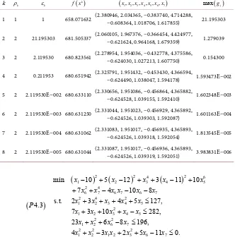
7 2 2.119530E−004 680.631062 (2.331083, 1.951017, −0.456935, 4.365893, −0.624526, 1.039318, 1.592054) 1.813545E−005
8 2 2.119530E−005 680.631044 (2.331087, 1.951017, −0.456936, 4.365893, −0.624526, 1.039319, 1.592051) 3.983831E−006
(
)
(
)
2(
)
2 4(
)
2 61 2 3 4 5
2 4
6 7 6 7 6 7
2 4 2
1 2 3 4 5
2
1 2 3 4 5
2 2
1 2 6 7
2 2 2
1 2 1 2 3 6 7
min 10 5 12 3 11 10
7 4 10 8
s.t. 2 3 4 5 127,
4.3
7 3 10 282,
23 6 8 196,
4 3 2 5 11 0.
x x x x x
x x x x x x
x x x x x
P
x x x x x
x x x x
x x x x x x x
− + − + + − +
+ + − − −
+ + + + ≤
+ + + − ≤
+ + − ≤
+ − + + − ≤
[image:12.595.208.540.366.709.2]DOI: 10.4236/ojop.2019.84010 125 Open Journal of Optimization
(
)
(
1 2 3 4 5 6 7)
, , , , , ,
2.330499,1.951372, 0.4775414,4.365726, 0.6244870,1.038131,1.594227 x x x x x x x
= − −
with the optimal objective function value 680.6300573. Let x0=
(
1,2,0,4,0,1,1)
, 1 1ε = , ρ =1 1,
η
=0.1, andσ
=2 in Algorithm 3.2. We chooseδ
=0.00001for
δ
-feasibility. Numerical results for (P4.3) are given in Table 3, where forTable 3 we use a Gradient-type algorithm to solve the subproblem in Step 2. From the above classical examples, we can see that our approximate algorithm can produce the approximate optimal solutions of the corresponding problem successfully. But the convergent speed can be improved if we use the New-ton-type method in Step 2 of Algorithm 3.2, which will be researched in our fu-ture work.
Funding
This research is supported by the Natural Science Foundations of Shandong Province (ZR2015AL011).
Conflicts of Interest
The author declares no conflicts of interest regarding the publication of this pa-per.
References
[1] Zangwill, W.I. (1967) Nonlinear Programming via Penalty Function Management.
Science, 13, 334-358.https://doi.org/10.1287/mnsc.13.5.344
[2] Di Pillo, G., Liuzzi, G. and Lucidi, S. (2011) An Exact Penalty-Lagrangian Approach for Large-Scale Nonlinear Programming. Optimization, 60, 223-252.
https://doi.org/10.1080/02331934.2010.505964
[3] Han, S.P. and Mangasarian, O.L. (1979) Exact Penalty Functions in Nonlinear Pro-gramming. Mathematical Programming, 17, 251-269.
https://doi.org/10.1007/BF01588250
[4] Ben-tal, A. and Teboulle, M. (1989) A Smoothing Technique for Non-Differentiable Optimization Problems. Lecture Notes in Mathematics, Springer Verlag, Berlin, Vol. 1405, 1-11.https://doi.org/10.1007/BFb0083582
[5] Herty, M., Klar, A., Singh, A.K. and Spellucci, P. (2007) Smoothed Penalty Algo-rithms for Optimization of Nonlinear Models. Computational Optimization and Applications, 37, 157-176.https://doi.org/10.1007/s10589-007-9011-6
[6] Pinar, M.C. and Zenios, S.A. (1994) On Smoothing Exact Penalty Functions for Convex Constarained Optimization. SIAM Journal on Optimization, 4, 486-511. https://doi.org/10.1137/0804027
[7] Auslender, A., Cominetti, R. and Haddou, M. (1997) Asymptotic Analysis for Pe-nalty and Barrier Methods in Convex and Linear Programming. Mathematics of Operational Research, 22, 43-62.https://doi.org/10.1287/moor.22.1.43
[8] Gonzaga, C.C. and Castillo, R.A. (2003) A Nonlinear Programming Algorithm Based on Non-Coercive Penalty Functions. Mathematical Programming, 96, 87-101. https://doi.org/10.1007/s10107-002-0332-z
DOI: 10.4236/ojop.2019.84010 126 Open Journal of Optimization Computational Optimization and Application, 55, 155-172.
https://doi.org/10.1007/s10589-012-9504-9
[10] Lian, S.J. (2012) Smoothing Approximation to L1 Exact Penalty Function for
In-equality Constrained Optimization. Applied Mathematics and Computation, 219, 3113-3121.https://doi.org/10.1016/j.amc.2012.09.042
[11] Chen, C. and Mangasarian, O.L. (1995) Smoothing Methods for Convex Inequali-ties and Linear Complementarity Problems. Mathematical Programming, 71, 51-69. https://doi.org/10.1007/BF01592244
[12] Wu, Z.Y., Lee, H.W.J., Bai, F.S. and Zhang, L.S. (2017) Quadratic Smoothing Ap-proximation to L1 Exact Penalty Function in Global Optimization. Journal of In-dustrial and Management Optimization, 1, 533-547.
https://doi.org/10.3934/jimo.2005.1.533
[13] Meng, Z.Q., Dang, C.Y. and Yang, X.Q. (2006) On the Smoothing of the Square-Root Exact Penalty Function for Inequality Constrained Optimization. Computational Optimization and Applications, 35, 375-398.
https://doi.org/10.1007/s10589-006-8720-6
[14] Wu, Z.Y., Bai, F.S., Yang, X.Q. and Zhang, L.S. (2004) An Exact Lower Order Pe-nalty Function and Its Smoothing in Nonlinear Programming. Optimization, 53, 51-68.https://doi.org/10.1080/02331930410001662199
[15] Lian, S.J. (2016) Smoothing of the Lower-Order Exact Penalty Function for Inequa-lity Constrained Optimization. Journal of Inequalities and Applications, 2016, Ar-ticle No. 185.https://doi.org/10.1186/s13660-016-1126-9
[16] Liu, B.Z. (2009) On Smoothing Exact Penalty Functions for Nonlinear Constrained Optimization Problems. Journal of Applied Mathematics and Computing, 30, 259-270.https://doi.org/10.1007/s12190-008-0171-z
[17] Mangasarian, O.L. and Fromovitz, S. (1967) The Fritz John Necessary Optimality Conditions in the Presence of Equality and Inequality Constraints. Journal of Ma-thematical Analysis and Applications, 17, 37-47.
https://doi.org/10.1016/0022-247X(67)90163-1
[18] Hock, W. and Schittkowski, K. (1981) Test Examples for Nonlinear Programming Codes. Lecture Notes in Economics and Mathematical Systems, Vol. 187, Sprin-ger-Verlag, Berlin, Heidelberg, New York.