Bayesian Lifetime Modeling for Power Semiconductor Devices

Bayesian Lifetime Modeling for Power

Semiconductor Devices

Olivia Bluder

Alfred Waukmann

Abstract— Modeling and predicting lifetimes of smart power ICs has become more and more impor-tant during the last years. Higher demands on relia-bility and economy require prediction methods which save time and money. In this work two modeling ap-proaches are discussed: (a) Bayesian linear models and (b) Bayesian linear models with mixed distribu-tions. Both are based on the test parameters and include prior information. The information for the parameters of the prior distributions is taken from previous tests and the prior distribution itself is se-lected with help of global and local sensitivity analy-sis.

Keywords: Bayesian inference, linear models, semi-conductor lifetime

1

Introduction

In semiconductor industry the reliability of a device is es-sential, but gaining this information is not always straight forward. For the decision whether a device fulfills the re-quirements, lifetime tests are necessary. These tests are time and cost consuming, therefore reliable methods for predicting lifetime are needed.

The measured lifetimes of the devices under test (DUT) can not be modeled with known acceleration models like Arrhenius or Coffin Manson[1], therefore Bayesian Linear Models (LM) are used. The advantages of this method are: (a) available prior knowledge of previously measured data is integrated into the model, so not only current data have an impact on the model parameters. (b) higher flex-ibility and more information in the prediction.

In the first part the data and their characteristics will be described. Then follows the model definition, the prior selection and the global and local sensitivity analysis. In the last part of this work an advanced model is investi-gated and an outlook for further investigation topics will

∗_{Alpen-Adria-Universit¨at Klagenfurt, Universit¨atsstr.}

65-67, 9020 Klagenfurt, Austria, Tel: 0043-4242-34890-19, Email: [email protected]

†_{KAI - Kompetenzzentrum f¨ur Automobil- und}

Industrieelek-tronik GmbH, Europastrasse 8, 9524 Villach, Austria

‡_{Carinthia University of Applied Sciences, Europastr. 4, 9524}

Villach, Austria, Email: [email protected]

This work was jointly funded by the Federal Ministry of Economics and Labour of the Republic of Austria (contract 98.362/0112-C1/10/2005) and the Carinthian Economic Promotion Fund (KWF) (contract 18911|13628|19100)

be presented.

2

Used Data

For this study datasets containing lifetimes of Smart Power ICs [2], tested with a temperature cycle stress test system [3] at KAI, have been used. Smart means that each device includes several protection functions against over-temperature, over-current, open load, etc. These de-vices are frequently used in automotive applications, e.g. to replace mechanical relays.

The power switches have been tested under different elec-trical stress conditions. The test system measures and records the state of every DUT. The Cycles to Failure (CTF) of each DUT are determined by the test parame-ters. The four most important parameters are:

• clamping voltage (VCl[V]) • peak current ( ˆI[A])

• pulse length (tp[μs])

• repetition time (frequency) (trep[ms])

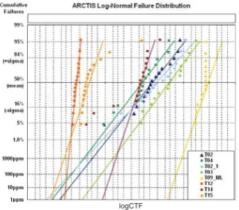
The model is based on 8 tests, all with the same device type and the same package. In these tests the four above mentioned test parameters have been changed. Accord-ing to previous investigations [4] it is known that the data follow a log-normal distribution, hence on the x-axis the logarithmic CTFs and on the y-axis the quantiles of the normal distribution are plotted to achieve linearity. The lifetimes of the DUTs for each test are shown in figure 1.

The gap between the first two tests (T12, T15) and the others is not attributable to significantly higher stress. This leads to the assumption that two failure mechanisms are dominating. To verify this, devices from both groups have been sent to the failure analysis (FA) with the re-sults shown in figure 2.

logCTF

Figure 1: Results of tests

1st_{group 2}nd_group

Figure 2: FA pictures

As a first modeling approach a linear model (LM) will be used, in section 7 the assumption of two failure mecha-nisms will be integrated into the model, which implies a mixture of two distributions.

3

Bayesian Linear Model Theory

Bayesian LMs are derived from the Bayesian law[5], which is:

p(θ|y) =p(y|θ)·p(θ)

p(y) (1)

with p(θ|y) the posterior distribution (the distribution of the model parameters (θ) after measuring the CTF),

p(y|θ) the joint probability for the given data vector y

and the model parameters,p(θ) the prior distribution of the model parameters (before measuring the CTF) and

p(y) the probability of the given data, which can be ne-glected under the assumption of proportionality, because it is constant. Furthermore the joint probability can be expressed by the likelihood function (L(·)) of the data. The likelihood is the product of the probabilities of each value (yi) from the given set of dataydependent on the

model parameters (θ):

L(θ|y) =

n

i=1

p(yi|θ) (2)

hence the Bayesian law converts to:

p(θ|y)∝L(θ|y)·p(θ) (3)

which states that the posterior distribution is propor-tional to the product of the likelihood of the data and the prior distribution of the model parameters. In the prior distribution the information of previous tests will be included.

LMs can be used for normal distributed data. Since the given data follow a log-normal distribution, a loga-rithmic transformation leads to normal distributed data. The transformed data (log₁₀CT F = y) are normal dis-tributed with μthe vector of means and Σ =σ2I (vari-ance times identity matrix) the covari(vari-ance matrix:

y∼N(μ, σ2I) = (2πσ2)−12_exp−2σ12(y−μ)(y−μ) ₍₄₎

Next the dependency on the four test parameters (the covariates) is integrated into the model by using a LM for the meanμ:

μ=βX=β0+β1∗VCl+β2∗Iˆ+β3∗tp+β4∗trep+ (5)

whereX is the matrix of normalized covariates and with

∼N(0, σ2I) the random errors.

Combining equations 4 and 5 leads to a likelihood func-tion dependent on a total of six model parameters:

L(β, σ2|X, y) = (2πσ2)−n2 _exp−2σ12(y−Xβ)(y−Xβ) ₍₆₎

4

Prior Selection

Selecting the prior distribution is essential for Bayesian inference, because the influence on the posterior distri-bution of the parameters can be significant. If there is no scientific reason for selecting one dedicated prior dis-tribution, basically there is no restriction for it, even an improper prior (does not fulfill the conditions for a dis-tribution function) can be used. Nevertheless, selection must be made carefully because a bad prior can lead to a bias in the model.

Prior selection can be supported by global sensitivity analysis, a method for comparing resulting posterior dis-tributions of possible prior disdis-tributions. In this work a set of uninformed and informed priors is used. Unin-formed means that no knowledge about the parameters is given, informed means knowledge, e.g. mean and stan-dard deviation, from given data or from experts is avail-able.

Possible distributions for theβis are the following:

• diffuse normal: βi∼N(0,106)

• informed uniform: βi∼U(mi−3∗si, mi+ 3∗si) • informed normal: βi∼N(mi, s2i)

• non centralized student t with 1 df: βi∼nct(mi,1) • gamma or negative gamma distributions: βi ∼

±Gam(ai, bi)

The prior information for the means m = (6.71,−13.85,−23.88,−16.41,6.28) and the standard deviations s = (0.13,1.04,1.65,1.15,0.93) of the model parameters are extracted from the given data.

When normal priors for the βis and an inverse gamma

(IG) prior for σ2 are used, than the resulting posterior distributions for the parameters can be calculated analytically (βi|y ∼ t and σ2|y ∼ IG), but in all other

cases the posterior distribution needs to be simulated numerically. This has been done with the slice sampling algorithm in MATLAB1, with a sample size of 10000 and a burn in period of 1000.

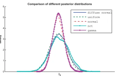
The densities of the resulting posterior distributions for the five β parameters show similar characteristics, therefore only β0 is visualized in figure 3. The global

sensitivity analysis shows a division into two groups. Densities with less variation descend from highly in-formed priors (gamma and normal) and the flatter ones from diffuse and little informed priors (diffuse normal, uniform and non-centralized t). Furthermore, the posteriors differ only in shape not in location, this means that all assumed prior distributions are acceptable, but the choice for the degree of information integrated needs to be made.

1_{MATLAB R2008, MathWorks}

For calculating the parameters of the prior distributions reliable data have been used and it is intended that the prior contains as much information as possible without manipulating the results, hence an informed normal distribution will be used as prior.

σ2 requires a global sensitivity analysis too. As possible priors informed lifetime distributions (inverse gamma, log-normal and Weibull) are considered, because they are restricted to R+. For completeness also a diffuse normal and a uniform prior are used. Although the shapes and the degrees of information of the used priors differ significantly, the influence on the posterior distri-bution of σ2 is negligible. Therefore the inverse gamma distribution will be used, because it is the conjugate prior for normal distributed data. In Bayesian modeling conjugate means that the posterior distribution is from the same family as the prior distribution[5].

After selecting a proper prior local sensitivity analy-sis needs to be performed, this means evaluating if the posterior distribution is sensitive to reasonable changes in the parameters of the prior distribution. Sensitive posteriors can lead to big variations in the model and poor prediction quality will be the result. Reasonable changes according to Gill [5] are shifts in prior mean of plus/minus one prior standard deviation respectively multiplying/dividing the prior standard deviation by two. If the resulting posterior of the transformed prior shows significant differences in location or shape, a less informed prior for this parameters should be chosen.

Figure 4 shows the resulting posterior densities of two parameters after local sensitivity analysis. Only β0 and

σ2 are visualized, since they show the biggest variations. The results shown in figure 4 indicate that shifting the mean has only slight influence on the posterior distribu-tion. Using a transformed standard deviation has no in-fluence onσ2, but reducing the prior standard deviation of β0 by 50% leads to a reduce of 25% in the posterior

distribution, hence this posterior distribution is sensitive to transformations. This problem can be solved by using a less informed prior (e.g. use two times the variance). With this modificated prior the effect for the mean re-duces and the sensitivity to transformations in the stan-dard deviation vanishes.

5

Model Definition

After selecting the prior the full Bayesian LM can be defined as:

y ∼ N(μ, σ2I)

μ = Xβ+

βi ∼ N(mi, si)

σ2 ∼ IG(a, b) (7)

likeli-0 1 2 3 4 5

β₀

density

diffuse normal

uniform

normal

nct

gamma

Figure 3: Simulated posterior distributions forβ0

0 1 2 3 4 5 6

density

Sensitivity analysis for posterior distributions

μ μ − σ μ + σ

0 2 4 6 8 10

σ2

density

β0

μ μ − σ μ + σ

0 2 4 6 8 10

σ2

density

σ σ/2 σ*2 0

2 4 6 8

β0

density

σ σ/2 σ*2

Figure 4: Results of local sensitivity analysis

hood times the prior distribution of the parameters. In-tegrating the specific joint posterior distribution of the model defined in equation 7 with respect toβandσ2, re-spectively, leads to student t distributions for theβis and

to an inverse gamma distribution forσ2. The summary statistics for the model parameters are given in table 1.

Table 1: Summary statistics of posterior distributions Quantiles parameter mean st.dev 5% 95%

β0 (intercept) 6.71 0.08 6.58 6.84

β1 -13.82 0.91 -15.30 -12.32

β2 -24.03 1.14 -26.02 -22.21

β3 -16.38 0.73 -17.61 -15.22

β4 6.38 0.54 5.54 7.29

σ2 0.71 0.05 0.64 0.79

The standard deviations of the model parameters vary between 1-8% of the mean and the percentages of the simulation errors are in the same range, this means that simulation results are reliable, although they might be improved since<5% simulation error is desired.

6

Posterior Predictive Distribution

The main intention for finding an appropriate model for CTFs of semiconductor devices is to predict reliable life-times. In case of Bayesian LMs predictions are no point

estimates but posterior predictive distributions of the data. The output is the distribution of new data after observing and including the information of the old data. For a given set of new data (ynew), the posterior

predic-tive distribution is[5]:

p(ynew) =

Θp(ynew, θ|Y)dθ

=

Θ

p(ynew, θ|Y)

p(θ|Y) p(θ|Y)dθ

=

Θp(ynew|θ, Y)p(θ|Y)dθ (8)

which is the integral over the product of the joint prob-ability of data and model parameters (p(ynew|θ, Y))

and the posterior distribution of the model parameters (p(θ|Y)). For the Bayesian LM defined in equation 7 with a new set Xnew of covariates the posterior

predic-tive distribution of the resulting log₁₀CT F (= ˜y) is:

p(˜y) =

Θp(˜y|β, σ

2_{, X}

new, X, y)p(β, σ2|X, y)dθ (9)

In special cases this distribution can be calculated, but since simulation data of the involved distributions are available, sampling from them is also a solution.

0 0.05 0.1 0.15 0.2 0.25 0.3 0.35 0.4 0.45 0.5

logCTF

density

Comparison of data and posterior predictive distributions

failed =0.01%

data post. pred. dist

0 0.1 0.2 0.3 0.4 0.5 0.6 0.7

logCTF

density

failed =100%

data post. pred. dist

T02 T15

Figure 5: Comparison of predicted and real density of two datasets

10000) and the percentage of failed tests is the indica-tor for the model quality The comparison of the pre-dicted and the real density of two representative datasets is shown in figure 5. The used model fits the data of test

T02 almost perfectly, because only 0.01% of the GoF tests fail. In contrast to this result 100% of the GoF tests fail for test T15. In total, three posterior predic-tive distributions fit the data well (failed GoF < 3%), two show weaknesses (failed GoF≈35%) and three show poor fitting quality (failed GoF> 87%).

One reason for bad quality in the five cases was already mentioned in section 2. The data show a division into two groups with different failure mechanisms and additionally a transition zone, this means that some datasets belong to both groups, e.g. T14. The mathematical reasons for bad model quality for these tests are:

• T12 andT09 have smallerσ2than other tests

• T05,T14 andT15 do not behave “well”, they show a mixture of two distributions

This implies that the model fits well for datasets of the second group in figure 1. Calculating the posterior pre-dictive distribution of the next two performed tests (T13 andT16), which are mainly part of the second group, ver-ifies the assumption. The percentage of failed GoF tests is 0% and 5%, respectively. This means the predicted values are reasonable.

The investigations show that the proposed Bayesian LM can be used for lifetime tests which are part of the sec-ond group, but model improvement is needed since weak-nesses for the first group of tests are observed. One so-lution is to adapt the model more to the mixed behavior of the data, this will be addressed in the next section.

7

Bayesian Linear Models with Mixed

Distribution

In section 2 the theory about two dominating failure mechanisms was introduced. This assumption leads to the idea of using Bayesian LM with a mixture of dis-tributions for this data. The used model consists of a combination of two normal distributions with a mixing proportion (π), this is:

y∼π∗N(μ1, σ1) + (1−π)∗N(μ2, σ2) (10)

where μ1 andμ2are modeled with LMs:

μ1 = β∗X

μ2 = γ∗X (11)

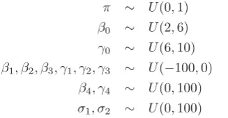
Using this model more than doubles the number of model parameters, i.e. from 6 to 13. The simulation with diffuse priors showed high variations in the model parameters, therefore less informed priors than for the Bayesian LM will be considered, these are uniform distributions on a pessimistically chosen interval. The information for the intervals is extracted from the performed tests, the ob-servations in figure 1 and the previously used Bayesian LM. This leads to the following priors:

π ∼ U(0,1)

β0 ∼ U(2,6)

γ0 ∼ U(6,10)

β1, β2, β3, γ1, γ2, γ3 ∼ U(−100,0)

β4, γ4 ∼ U(0,100)

σ1, σ2 ∼ U(0,100) (12)

The prior distributions of β0 and γ0 contain the

infor-mation that 106seams to be the border between the two groups, π is a weighting parameter, hence it has to be chosen from the interval [0,1] and the priors of the other parameters only restrict the sign.

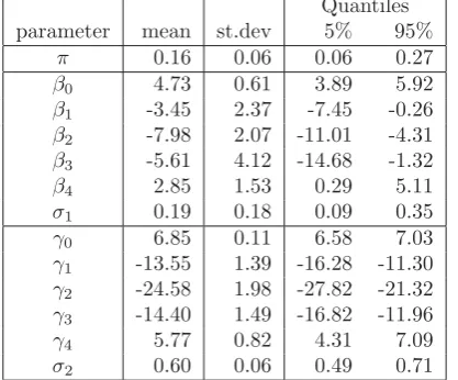
The simulation results (see table 2) show that the model parameters of the first distribution (βi’s andσ1) tend to

vary more than the others. A possible explanation is the lack of data, because out of the 123 data points only 35 are part of the first group.

The intention for using a mixture of distributions was to increase the quality of the model, but the higher variation in the parameters is already an indicator that the model will not fulfill the expectations.

0 0.1 0.2 0.3 0.4 0.5 0.6 0.7

logCTF

data predict LM predict Mixed LM

0 0.1 0.2 0.3 0.4 0.5 0.6 0.7

logCTF

data predict LM predict Mixed LM

Figure 6: Comparison of predictions of the two LMs investigated

Table 2: Summary statistics of posterior distributions for model with mixed distribution

Quantiles parameter mean st.dev 5% 95%

π 0.16 0.06 0.06 0.27

β0 4.73 0.61 3.89 5.92

β1 -3.45 2.37 -7.45 -0.26

β2 -7.98 2.07 -11.01 -4.31

β3 -5.61 4.12 -14.68 -1.32

β4 2.85 1.53 0.29 5.11

σ1 0.19 0.18 0.09 0.35

γ0 6.85 0.11 6.58 7.03

γ1 -13.55 1.39 -16.28 -11.30

γ2 -24.58 1.98 -27.82 -21.32

γ3 -14.40 1.49 -16.82 -11.96

γ4 5.77 0.82 4.31 7.09

σ2 0.60 0.06 0.49 0.71

8

Conclusions and Future Work

This work showed that modeling the lifetimes of power semiconductor devices with Bayesian LMs is possible, but restricted to a specific range, where tested devices have the same failure mechanisms. Expanding the prediction range showed the poor extrapolation quality of the model for tests with probably other failure mechanisms. As a step of improvement a Bayesian LM with mixed distri-butions was used, but no significant increase in quality could have been observed, hence further improvements and/or other model assumptions are needed.

Among all possible new or advanced approaches four have been chosen to be the most promising for the given data, these are:

• include accurate temperature measurements

• using non-linear models and incorporate known physical relationships and models for parameters

• add more prior information into the Bayesian LM with mixed distributions, e.g. model the mixing pro-portion (π) dependent on a parameter

• consider censored data (adapt the likelihood func-tion)

References

[1] Escobar, L. A., Meeker, W. Q., “A Review of Ac-celerated Test Models, Statistical Science, V21, N4, pp. 552-577, 11/06

[2] Glavanovics, M., Estl, H., Bachofner, A., “Reliable Smart Power Systems ICs for Automotive and In-dustrial Application - The Infineon Smart Multi-channel Switch Family”, 43. International Confer-ence Power Electronics, Intelligent Motion, Power Quality (PCIM 2001), N¨urnberg, Germany, 6/01 [3] Glavanovics, M., K¨ock, H., Eder, H., Koˇsel, V.,

Smorodin, T., “A new cycle test system emulat-ing inductive switchemulat-ing waveforms”, 12th European Conference on Power Electronics and Applications (EPE 2007), Aalborg, Denmark, pp.1-9, 9/07 [4] Bluder, O., “Statistical Analysis of Smart Power

Switch Life Test Results”, Diploma thesis, Alpen-Adria-University of Klagenfurt, Austria, March 2008

[5] Gill, J.,Bayesian methods, Chapman & Hall/CRC, Boca Raton FL, 2008.

[6] Hamada, M. S., Wilson, A. G., Reese, C. S., Martz, H. F.,Bayesian Reliability, Springer Science + Busi-ness Media, New York, 2007.