doi:10.4236/jssm.2010.31006 Published Online March 2010 (http://www.SciRP.org/journal/jssm)
Evolution or Revolution of Organizational
Information Technology – Modeling
Decision Makers’ Perspective
Niv Ahituv1*, Gil Greenstein2
1Faculty of Management, Tel Aviv University, Tel Aviv, Israel; 2Faculty of Technology Management, Holon Institute of Technology,
Holon, Israel; *Corresponding Author. Email: [email protected], [email protected]
Received December 28th, 2009; revised January 28th, 2010; accepted February 21st, 2010.
ABSTRACT
This paper suggests a new normative model that attempts to analyze why improvement of versions of existing decision support systems do not necessarily increase the effectiveness and the productivity of decision making processes. More-over, the paper suggests some constructive ideas, formulated through a normative analytic model, how to select a strategy for the design and switching to a new version of a decision support system, without having to immediately run through a mega conversion and training process while temporarily losing productivity. The analysis employs the in-formation structure model prevailing in Inin-formation Economics. The study analytically defines and examines a system-atic informativeness ratio between two information structures. The analysis leads to a better understanding of the per-formances of decision support information systems during their life-cycle. Moreover, this approach explains norma-tively the phenomenon of “leaks of productivity”, namely, the decrease in productivity of information systems, after they have been upgraded or replaced with new ones. Such an explanation may partially illuminate findings regarding the phenomenon known as the Productivity Paradox. It can be assumed that the usage of the methodology that is presented in this paper to improve or replace information structure with systematically more informative versions of information structures over time may facilitate the achievement of the following major targets: increase the expected payoffs over time, reduce the risk of failure of new versions of information systems, and reduce the need to cope with complicated and expensive training processes.
Keywords: Decision Analysis, Decision Support Systems, Productivity and Competitiveness, Information Technology Productivity, the Productivity Paradox
1. Introduction
A major and continuing problem in the information te- chnology (IT) profession is the high rate of failure of new information systems (IS) or upgraded versions of them. From a rational point of view it may be assumed that IS professionals usually analyze and design IS “pro- perly”. But is it really so? Are they aware of the possibil-ity of limits in perception among IS users, especially decision makers? Do they realize that “improvement” of decision support information systems might lead some-times to a result opposite to what has been expected, namely degradation in the level of the productivity of the firms, since new and unfamiliar decision rules have not been fully implemented and adopted by the decision- makers?
This article suggests a new normative model that
at-tempts to explain that improvement of versions of exist-ing information systems do not necessarily increase the effectiveness and productivity of decision making proc-esses. It also suggests some constructive ideas, formu-lated through a normative analytic model, how to select a strategy of switching to new version of a system, without having to immediately run through a mega training pro-gram, and to take a risk of losing productivity.
The methodological and theoretical foundations for the analysis presented here anchor in the literature on infor-mation economics. The earliest mathematical model pre-senting the relaying of information in a quantitative form was that of Shannon [1]. The model distinguished be-tween two situations:
1) A noise-free system—a univalent fit between the transmitted input data and the received signals;
(denot-ing a state of nature) are translated into signals probabil-istically.
In assigning an expected normative economic value to information, some researchers made use of Microeco-nomics and Decision Theory tools [2]. The combination of utility theory and the perception that information sys-tems can be noisy led to the construction of a probabilis-tic statisprobabilis-tical model that accords to an information system the property of transferring input data (states of nature) to output (signals) in a certain statistical probability [3–5]. This model, which delineates a noisy information system, is called the information structure model. It is based on
the assumption that a system is noisy but it does not ex-amine the nature of the noise. This paper expands the analysis by examining some patterns of noise. The con-sequences of that analysis are then demonstrated.
Over the years significant research was conducted to explore aspects of the phenomenon termed by Simon [6] as “bounded rationality”1 and its main derivative—sa- tisficing behavior. Some of its aspects were presented
comprehensively by Rubinstein [7]. Ahituv and Wand [8] showed that when satisficing is incorporated into the information structure model, there might be a case where none of the optimal decision rules will be pure anymore (unlike the results of optimizing behavior).
Ahituv [9] incorporated one of the aspects of bounded rationality into the information structure model: the in-ability of decision-makers to adapt instantaneously to a new decision rule when the technological characteristics of the information system, as expressed by the probabili-ties of the signals, are suddenly changed. Moreover, Ahi- tuv [10] portrayed a methodology in which decision support systems are designed to act consistently during their lifecycle (in accordance with a constant decision rule). He suggested that this decision rule (that was an optimal decision rule in a previous version of the infor-mation system) guarantees improvement of expected outcomes, although it is not necessarily the optimal deci-sion rule for later verdeci-sions of this information system.
This study presents a conceptual methodology that combines aspects of bounded rationality [9,10] dealing with a rigid decision rule and the life-cycle of informa-tion systems, with elements of rainforma-tional behavior pre-sented in the information structure model [5].
The article raises some questions: Is it possible to im-prove an existing information system without adopting a new decision rule? What are the analytical conditions that enable a “smooth” (without much disturbance) up-grading or replacement of an information system? In a
decision situation where two information structures are activated probabilistically, and one of them is generally more informative than the other, are there analytical con-ditions encouraging to enhance the percentage of usage of the superior system?
A normative framework is suggested to cope with es-sential processes (e.g.: implementation processes, correc-tion of bugs, or upgrading of versions) during the life cycle of a decision support system [11]. By defining and analyzing a new informativeness relationship - “the sys-tematic informativeness ratio”, this paper demonstrates situations where decision-makers are equipped with par-tial information. Through these cases, it is explained how to assure a “smooth” implementation of new or upgraded information systems, as well as how to reduce the in-vestment in implementation activities.
Moreover, It is shown that the existence of this new relationship (ratio) between two information structures enables to improve the level of informativeness without the awareness and the involvement of the users (the deci-sion makers).
“The systematic informativeness ratio approach”, whi- ch is presented and analyzed for the first time in this pa-per, contributes to better understanding of various as-pects of the “productivity paradox” [12–14]. Furthermore, it portrays a methodology that suggests how to deal with some aspects of the “productivity paradox” which were explored in earlier studies [15,16].
The next section summarizes the information structure model and the Blackwell Theorem [5]. It describes the motivation to use convex combinations in order to de-scribe processes during the life cycle of a decision sup-port system. Section 3 describes, analyzes, and demon-strates a new informativeness relationship between two
information systems—“the systematic informativeness
ratio”. Section 4 explores the existence of systematic
informativeness ratio between un-noisy information str- uctures. Section 5 presents some implications that could be extrapolated to noisy information structures. The last section provides a summary and conclusions, and pre-sents the contribution of the study and the directions it opens for further research. Proofs of the theorems and lemmas appear in the appendix.
2. The Basic Models
2.1 The Information Structure Model and Blackwell Theorem
The source model employed in the forthcoming analysis is the information structure model [5]. This is a general model for comparing and rank ordering information sys-tems based on the rules of rational behavior.2
The information structure model enables a comparison of information systems using a quantitative measurement reflecting their economic value. An information structure
1Simon termed the human decision-making process, which is affected
Q1 is said to be more informative than an information
structure Q2 if the expected payoff of using Q1 is not
lower than the expected payoff of using Q2. The expected
payoff is trace (*Q*D*U)3, where trace is an operator
that sums the diagonal elements of a square matrix. The objective function for maximizing the expected compen-sation is Max
trace( Q D U)
D * * *
4.
Let us examine a numerical example. Assume that an investment company serves its customers by using a web
based information system. Let Q1 be an information
structure that predicts the attractiveness of investing in various alternative channels. The IS supports the deci-sion-making of the investors. For simplicity, suppose there are three categories of states of nature: S1 -
acceler-ated growth (probability: 0.2), S2 - stability (probability:
0.6), and S3- recession (probability: 0.2). Assume also
that there are three possible decisions: A1 - Invest in bank
deposits; A2 - Invest in stocks; A3- Invest in foreign
cur-rency; Q1- The information system provides the
follow-ing signals: Y1- Accelerated growth is expected; Y2-
Sta-bility is expected; Y3 - Recession is expected;
1 0 0 0 6 . 0 4 . 0 0 4 . 0 6 . 0 1 Q
The compensations matrix U, which represents the
expected percentage of profit or loss, is described as
fol-lows: 3 1 1 0 5 0 1 0 3 U
4 . 2 3 1 1 0 5 0 1 0 3 1 0 0 0 6 . 0 4 . 0 0 4 . 0 6 . 0 2 . 0 0 0 0 6 . 0 0 0 0 2 . 0 * * * 3 , 3 2 , 3 1 , 3 3 , 2 , 2 1 , 2 3 , 1 2 , 1 1 , 1 2 1 D D D D D D D D D U) D Q trace( Max D where 1 0 0 0 0 1 0 0 1 *D 5. Invest “A
1”, while the signal is
Y1 or Y2. Invest “A3”, while the signal is Y3.
Given two information systems that deal with the same state of nature and are represented by the information structures Q1 and Q2, Q1 is defined as generally more
in-formative6 Given two information systems that deal with
the same state of nature and are represented by the in-formation structures Q1 and Q2, Q1 is defined as generally
more informative.7 The rank ordering is transitive.8
Over the years, a number of researchers developed
analytical models to implement the concept of the
infor-mation structure model in order to evaluate the value of information technology. Ahituv [10], demonstrated the life cycle of decision support information system with the model. Ahituv and Elovici [17] evaluated the value of performances of distributed information systems. Elovici
2According to the information structure model, four factors determine
the expected value of information.
The a priori probabilities of pertinent states of nature. Let Sbe a finite set of n states of nature: S={S1,..,Sn}. Let P be the vector of a
priori probabilities for each of the states of nature: P=(p1,..,pn).
The information structure – a stochastic (Markovian) matrix that transmits signals out of states of nature. Let Y be a finite set of n sig-nals, Y={Y1,..,Ym}. An information structureQ is defined such that its elements obtain values between 0 and 1, Q: SxY[0,1]. Qi.j is the prob-ability that a state of nature Sii displays a signal Yj 1
1
m j i,j QThe decision matrix – a stochastic matrix that links signals with the decision set of the decision-maker. Let A be a finite set of k possible decisions, A={A1,..,Ak}. Let D be the decision function. Similar to Q, D
is a stochastic (Markovian) matrix, namely, it is assumed that the deci-sion selected for a given signal is not necessarily always the same. D:Y x A[0,1]
The payoff matrix – a matrix that presents the quantitative compensa-tion to the decision-maker resulting from the combinacompensa-tion of a decision chosen and a given state of nature. Let U be the payoff function: U :A x S (a combination of a state of nature and a decision provides a fixed compensation that is a real number). Ui,j – is the compensation yields when decision maker decides –“Ai”, while state of nature “Sj” occurs.
3Sometimes Q represents an un-noisy (noise free) information
struc-ture. In these cases Q represents an information function f, f:SY[4]. Q is a stochastic matrix that contains elements of 0 or 1 only. This means that for each state of nature the information structure will al-ways act identically (will produce the same signal), although it is not guaranteed that the state of nature will be exclusively recognized.
4When the utility function is linear, that is, the decision-maker is of the
type EMV [2], a linear programming algorithm may be applied to solve the problem, where the variables being the elements of the decision matrix D. It can be proved that at least one of the optimal solutions is in a form of a decision matrix whose elements are 0 or 1 (a pure decision rule), [5]. For numerical illustrations of the model, see [8–10].
5 *
D is a decision matrix which represent the optimal decision rules in this decision situation.
6It should be noted that when we deal with two information functions rather than structures we use the term “fineness” to describe the general informativeness ratio [4].
7In terms of the information structure model, if for every possible payoff matrix U, and for every a priori probability matrix
trace(*Q*D*U)
Max
trace(*Q*D*U)
Max
D
D 1 2 , then Q1 is generally
more informative than Q2, Denoted: Q1Q2. Blackwell Theorem
states that Q1 is generally more informative than Q2 if and only if there
is a Markovian (stochastic) matrix R such that Q1*R = Q2. Ris termed
the garbling matrix
et al [18] used this method to compare performances of Information Filtering Systems. Ahituv and Greenstein [15] used this model to assess issues of centralization vs. decentralization. Aronovich and Spiegler [19] use this model in order to assess the effectiveness of data mining processes.
The model was expanded to evaluate the value of in-formation in several aspects: the value of a second opin-ion [20]; the value of informatopin-ion in non-linear models of the Utility Theory [21]; analyzing the situation of case dependent signals (the set of signal is dependent on the state of nature, [22]); a situation of a two-criteria utility function [23]. The model was also implemented to evaluate empirically the value of information in postal services [24], and in analysis of Quality Control methods [25,26].
2.2 The Use of Convex Combinations9 of Information Structures to Represent Evolution during Their Life-Cycle
A possible reason why we should consider probabilistic combination of information systems is the existence of decision support systems that use Internet (or intranet) based search engines. These engines can retrieve infor-mation from several inforinfor-mation sources, and produce signals accordingly. The various sources are not always available.
Information sources are essential for the proper sur-vivability of competitive organizations. As a result, the importance of proper functioning of information systems is increasing. When a certain source in unavailable it is possible to acknowledge the users about it by alarming them with a special no-information signal [15]. Another option, which is presented in this paper, is to consider implementation of a “mixture” of information systems. For example: suppose there is “a state of the art” organ-izational information center that can serve, during peak times only 90% of the queries. How will the rest 10% are served? One alternative is to reject them.10 Another one is
to direct those queries to a simpler (perhaps cheaper) information system whose responses are less informative. This leads to consider probabilistic usage of information systems that can be delineated by a convex combination.
The analysis focuses on the convex combination of information structures reflecting a probabilistic employ-ment of a variety of information systems (structures), where the activation of each one of them is set by a given probability. The various systems react to the same states of nature and produce the same set of signals.11
The mechanism of convex combinations12 of
informa-tion systems is employed in an earlier research by Ahituv and Greenstein [15] which analyses the effect of prob-abilistic availability of information systems on produc-tivity, and illuminates some aspects of the phenomenon that are termed as “the productivity paradox” [12–14].
3. The Systematic Informativeness Ratio
3.1 Definition of the Systematic Informativeness Ratio
As mentioned in Section 2, when an information struc-ture Q1 is more informative than an information structure Q2 irrespective of compensations and a priori
probabili-ties, a general informativeness ratio exists between the two of them [5].
If an information structure Q1 is more informative than Q2 when the optimal decision rule of Q2 is employed, and
given some certain a priori probabilities of the states of nature, then under some assumptions on the payoffs, an informativeness ratio under a rigid decision rule is de-fined between them [9].13
9The convex combination of information structures was discussed in earlier studies. Marschak [4] notices that the level of informativeness of convex combination of two information structures (denoted Q1 and Q2)
which produce the same set of signals is not equivalent to the level of informativeness of using Q1 with a probability p and Q2 with the
com-plementary probability (1-p).
10Sulganik [27] indicates that a convex combination of information
structure could be used to describe experimental processes (with a probability p of success and (1-p) of failure). For example, he investi-gates the convex combination of two information structures: one pre-sents perfect information and the other one no-information (its rows are identical).
11It should be noted that in case that the two information structures do
not produce the same set of signals, the non-identical signals can be represented in by columns of zeroes respectively [9].
12A convex combination of two information systems is defined as
fol-lows: Let Q1 and Q2 be two information structures describing
informa-tion systems. Let S={S1,…,Sn} be their set of the states of nature. Let
Y={Y1,…,Ym} be their set of signals. When a decision situation is given
let p the probability that Q1 will be activated, and (1-p) that Q2will be
activated. Since, decision makers do not aware which information structure is activated, Q3, the weighted information structure, is
repre-sented by a convex combination of Q1 and Q2.
Q3= p* Q1 + (1-p) * Q2
13Given two information systems that deal with the same states of
na-ture, produce the same set of signals, and are represented by the infor-mation structures Q1 and Q2 respectively, Q1 will be considered more
informative than Q2 under a rigid decision rule if its expected payoff is
not lower than that of Q2 for the following conditions: .
,.., 1
,i n
i
Let U(k(i),i) the single maximum payoff when the state of natureSioccurs.
Denote:
* max( ( ( ), ); * min( ( ( ), );
u U k i i u U k i i
i i
0 max ( , ); 0 min ( , );
, ( ) , ( )
u Uk i u Uk i
i k k i i k k i
t (k(n)) 1(n, (k(1)),.., 1(1, *
1 (q q )
q
q2*(q2(1,(k(1)),..,q2(n,(k(n)))t, respectively.; * *
0
u
u
* u*u0; 0u0u0;
The theorem which is proved by Ahituv [9], states that:
If t(*q1**q2*)0 then Q1 more informative than Q2 with
regard to U and Π.
The ratio will be denoted: Q1 Q2
R
Assume those two informativeness ratios can be con-ceptually combined to a new informativeness ratio: Let
Q1 and Q2 be two information structures that deal with
the same state of nature and produce the same set of sig-nals. Q1 will be considered systematically more
informa-tive than Q2 if for any decision situation (for any a priori
probabilities vector- and any payoff matrix-U), its
expected payoff is not lower than that of Q2 while Q1
operates under an optimal decision rule of Q2. In terms of
the information structure model, this is presented herein-after by Definition 1.
Definition 1: Let Q1 and Q2 be two information
struc-tures representing two information systems operating on the same set of states of nature S = {S1,…,Sn} and pro-ducing the same set of signals Y = {Y1,…,Ym}. Q1 is
de-fined systematically more informative than Q2, denote
2 1 Q
Q S
, if for any decision situation (irrespective of
payoffs and a priori probabilities) Q1 is more informative
than Q2 under an optimal decision rule of Q2.
It means that if Q1is systematically more informative
than Q2, then for every decision situation14 there exists an
optimal decision rule of the inferior information structure
Q2, that can be used with the superior information
struc-ture Q1, and guarantees at least the optimal outcomes of
using Q2.
Mathematically it looks this way:
2
2 2 1 2
2 2
{ max ( )} ( )
( ( * )) ( ))
Q Q
Q D
D D Q ,traceΠ* Q * D * U
Max trace Q * D* U traceΠ* Q * D * U
where { max ( )}D Q2 - denotes the set of optimal deci-sion rules, when Q2 is activated in this specific decision situation.
In contrast to the general informativeness ratio, in the systematic informativeness ratio the information struc-ture Q2 can be replaced with the superior systematically
information structure Q1, without an immediate
aware-ness of the decision makers (the users), since the decision rule does not necessarily have to be changed instantane-ously. It means that when the systematic informativeness ratio exists between two information structures, at least the same level of expected payoffs is guaranteed when
the superior15 information structure is activated. Hence
the decision maker does not have to adopt a new optimal decision urgently.
Let us now examine the informativeness ratio between two information systems from the point of view of “sm- ooth” implementation. This is presented in Definition 2.
Definition 2: Let Q1 and Q2 be two information
struc-tures representing two information systems operating on
the same set of states of nature S={S1,…,Sn} and produc-ing the same set of signals Y={Y1,…,Ym}. Assume Q1 is
generally more informative than Q2. A smooth
imple-mentation of Q1 instead of Q2 is defined if for any level
of usage p
0p1
p*Q1(1p)*Q2Q2.The importance of this ratio is that in any probabilistic level of usage of the superior information system Q1, the
mean of the expected payoffs (compensation) that the decision-makers gain is not less than that achieved by using only the inferior information system. It contributes to a smooth implementation of the superior information structure Q1.
In our study we argue that those definitions (1 & 2) are equivalent. Theorem 1 proves analytically the equiva-lence of Definition 1 and 2.
Theorem 116
Let Q1 and Q2 be two information structures operating
on the same set of states of nature S = {S1,…,Sn}, and
producing the same set of signals Y = {Y1,…,Ym}. Then 2
1 Q
Q S
p,0 p1, p*Q1(1p)*Q2 Q2This theorem shows that the two ratios which have been defined above are identical. Replacement (or improvement, or upgrade) of an information structure with a more sys-tematically informative, information structure than it, guarantees smooth implementation, and vice versa.
Moreover, from the aforementioned equivalence it is understood that during a smooth implementation of the superior information structureQ1
17, we do not have to
adopt a new decision rule, and we can stick to an optimal decision rule we used in the past with the inferior infor-mation structureQ2. In fact this theorem sets a new
nor-mative perspective that defines the necessary and suffi-cient conditions for the ability to implement a superior information structure smoothly without immediate inter-ference in the routine work of decision makers.
Using this method facilitates information systems pro-fessionals to plan systems under the assumption that during a certain transition period the decision-makers may act identically and stick to the same decision-rule [10]. The existence of this informativeness ratio reduces the criticality of an urgent implementation process.
3.2 A Framework to Examine the Existence of the Systematic Informativeness Ratio
In order to identify the existence of a systematic infor-mativeness ratio between two information structures when one of them is generally more informative than the other, we would analyze a special case in which the number of signal and the number of states of nature are identical. In this case, the identity square matrix I is a complete and perfect information structure. We will try
to find out whether I is systematically more infor-
mative than any other square stochastic matrix of similar
14A given set of a-priori probabilities - Π, and a given utility matrix
- .U
15Systematically more informative than the other. 16The proof is provided in the appendix. 17Since
2 2 1 (1 )*
* , 1 0
, p p Q p Q Q
p
, Q1 Q2
S
dimensions.
The motivation to do this is provided by Lemma 1. Assume two information structures Q1 and Q2act on the
same set of states of nature, and respond with the same set of signals, and Q2Q1*R, where R is a stochastic
matrix (Blackwell Theorem’s condition). In Lemma 1 it is shown that the existence of systematic informativeness
ratio between I and R sets a pre-condition (sufficient
condition) to the existence of the general informativeness ratio between Q1 and Q2.
Lemma 118
Let Q1 and Q2 be two information structures operating
on the same set of states of nature S = {S1,…,Sn}, and producing the same set of signals Y = {Y1,…,Ym}. As-sume that Q1is generally more informative than Q2,
im-plying that Q2= Q1*R,whereRis a stochastic matrix [5]. If p,0 p 1, p I* (1 p)*R R ,
Then p,0 p1, p*Q1(1p)*Q2Q2
From Lemma 1 it can be shown that if Q1 is generally
more informative than Q2, namely Q2= Q1*R
(
R is a stochastic matrix) andS
I R (I is systematically more informative than R) then Q1 Q2
S
(Q1 is systematically
more informative than Q2).
3.3 The Monotony of the Systematic Informativeness Ratio
The following lemma deals with the improvement of the accuracy level of information systems by enhancing the probability to receive perfect information.
Lemma 219
Let I be an information structure that provides perfect
information. Let Q be any information operating on the
same set of states of nature S{S ,..,S 1 n} and producing the same set of signals Y = {Y1,…,Yn}.
If: for 0 p1,p*I(1p)*QQ (every convex
combination of I and Q is generally more informative
than Q) Then: q)*Q ( q*I p)*Q ( ,p*I p q
q,
0 1 1 1
Conclusion:
If: p, 0 p1,p*I(1p)*QQ Then: q)*Q ( q*I p)*Q ( ,p*I p q q,
p,
0 1 1 1
This lemma proves the monotony of the systematic informativeness ratio. Actually it is shown that an im-provement in the accuracy level of information (ex-pressed by increasing the probability of perfect
tion) is positively correlated with the general informa-tiveness ratio of a convex combination.
3.4 The Systematic Informativeness Ratio – An Example
We continue the example of Q1, an Information system
for choosing an investment option, which was first
dem-onstrated in Section 2.
1 0 0 0 6 . 0 4 . 0 0 4 . 0 6 . 0 1 Q
Suppose it is intended to replace the information
sys-tem with an improved one, Q2:
1 0 0 0 9 . 0 1 . 0 0 1 . 0 9 . 0 2 Q
Due to technological and organizational limitations, e.g.: inability to implement the system simultaneously all across the organization and the need to monitor carefully the system’s performances, the system is implemented step by step.
By using some of the lemmas and theorems presented above, it can be demonstrated that the information struc-ture Q2 is systematically more informative than Q1.
Let Q0 be an information system:
1 0 0 0 5 . 0 5 . 0 0 5 . 0 5 . 0 o Q
Let Q3 be an information structure, which represents
perfect information. 1 0 0 0 1 0 0 0 1 3 Q Since,
* 3 (1 )* 0
* 0 0, 1 0
, p p Q p Q Q Q
p
20 1 0 0 0 5 . 0 5 . 0 0 5 . 0 5 . 0 1 0 0 0 5 . 0 5 . 0 0 5 . 0 5 . 0 * 1 0 0 0 5 . 0 5 . 0 0 5 . 0 5 . 0 * ) 1 ( 1 0 0 0 1 0 0 0 1 * p p
then, from Theorem 1 it is clear that Q3 is systematically
more informative than Q0.
Let us present Q1 and Q2 as convex combination of Q3
and Q0.
0 3
2 0.8* 0.2*
1 0 0 0 9 . 0 1 . 0 0 1 . 0 9 . 0 Q Q
Q
18The proof and an example are provided in the Appendix. 19The proof is provided in the Appendix.
20We use the information structure Q0, as a garbling (stochastic) matrix,
1 0 0 0 5 . 0 5 . 0 0 5 . 0 5 . 0 * 2 . 0 1 0 0 0 1 0 0 0 1 * 8 . 0 1 0 0 0 5 . 0 5 . 0 0 5 . 0 5 . 0 * 8 . 0 1 0 0 0 1 0 0 0 1 * 2 . 0 * 8 . 0 * 2 . 0 1 0 0 0 6 . 0 4 . 0 0 4 . 0 6 . 0 0 3
1 Q Q
Q
According to Lemma 2 Q2is systematically more
in-formative than Q1. Table 1 demonstrates the implication
of the existence of the systematic informativeness ratio between Q2and Q1.
This example illustrates that if an upgrading of an in-formation system is based on the implementation of later versions of it which are systematically more informative than the earlier versions, then sticking to the old and fa-miliar decision rule will not harm productivity.
The principle of developing information systems to be systematically more informative provides the luxury of training and on-site implementation which is “life-cycle independence”. It facilitates the implementation of a new version of information system or insertion of minor changes, without the immediate awareness of the deci-sion makers. Therefore, organizations can schedule the optimal timing of wide training processes. That is in con-trary to the usual situation, when the scheduling of train-ing and on-site implementation might interfere with other organizational considerations and requirement (e.g.: pe- riodically tasks). Moreover, development of new deci-sion support systems without adopting this principle may
explain, normatively, “leaks of productivity”. In other words it may explain the decrease in user performance of information systems, although they have been improved. This degradation in the expected outcomes while using improved information systems can be attributed to the inability of users to adapt immediately to new decision rules.
4. The Systematic Informativeness
Ratio – A Noise Free Scenario.
4.1 Conditions for Existence of the Systematic Informativeness Ratio
Historically, the starting point for analyzing the value of information in noisy information structures was the ana- lysis of the value of information in noise free information
structures. These are also termed information functions
[4,5]. Following this approach, we will start with a sim-ple presentation of the informativeness ratio between in formation functions, which could be classified as un- noisy information structures.
In order to identify the existence of a systematic in-formativeness ratio between two information functions, a new aggregation ratio (a fineness ratio that keeps orders of signals) between information functions is defined, hereinafter.
Definition 3
Let fI be the identity information function. Let
} {S,..,Sn
S 1 be its set of states of nature and
} {Y ,..,Yn
Y 1 the set of signals fI produces. Hence,
Y S fI( i) i .
Assume for simplicity that S {1,..,n} , Y {1,..,n}
[image:7.595.92.251.90.230.2]then f iI( )i
Table 1. Comparison of two information structures, one of them is systematically more informative than the other
The current information structure
The improved information structure Information structure 1 0 0 0 6 . 0 4 . 0 0 4 . 0 6 . 0 1 Q 1 0 0 0 9 . 0 1 . 0 0 1 . 0 9 . 0 2 Q
The matrix of a priori probabilities for the states of nature + The matrix of compensation (percentage):
2 . 0 0 0 0 6 . 0 0 0 0 2 . 0 3 1 1 0 5 0 1 0 3 U
The Decision rules:
A1 – Invest in Bank Deposits
A2 – Invest in stocks
A3 – Invest in foreign currency
1 0 0 0 0 1 0 0 1 D 1 0 0 0 0 1 0 0 1 D 1 0 0 0 1 0 0 0 1 D
[image:7.595.63.539.514.710.2]Let Fbe a set of information functions that acts on
the same decision environment of
f
I .)
(
g(i) i or if g(i k i, then g(k) k Fg )
Since there is an isomorphism between the representa-tion of informarepresenta-tion funcrepresenta-tions and a set of informarepresenta-tion
structures representing them, Fcan be defined
analogi-cally as a set of un-noisy information structures.
) 1 1
1 1 1
1
1F(Fi,i or if Fi,k ,ki, then F k,k F
Following that fI is equivalent (for example) to I ,
an information structure that produces perfect information
I is represented by the identity Matrix of the order nxn.
In fact F is a complete set of information functions
that could be termed as aggregations of fI . If gFits way of transforming of states of nature into signals does
not contradict the way fI transforms states of nature
into signals. In other words it can be said that fI is a
higher resolution of every information function belong-ing to the set F.
Theorem 2 sets the necessary and sufficient conditions for the existence of systematic informativeness ratio
be-tween I (the identity information structure), and any
non-noisy information structure:
Theorem 221
Let F1 be an information function. Let S{S1,..,Sn} be its set of states of nature. Let Y{Y1,..,Yn} be its set
of signals. Let I be the identity information function,
which represent perfect information, then I F1
S
if and only if F1F.
It is shown in Theorem 2 that for every information function (non-noisy information structure) F1, the
neces-sary and sufficient condition that
I
is systematicallymore informative than F1, is that F12 F1. In fact,
four equivalent conditions are found as we will show below.
Let F1 be an information function. Let
,..,S S
S{ 1 n} be its set of states of nature. Let
} {Y ,..,Yn
Y 1 be its set of signals. The following
condi-tions are equivalent.22
1) I F1
S
2) p, 0 p1 p*I(1-p)*F1F1
3) F1F
4) F12F1
The equivalence of the first and second conditions (which was demonstrated earlier by Definition 1 and 2 respectively) was proven by Theorem 1. Conditions 1
and 2 are not specific to un-noisy information structures, and can hold for any type of structure. In contrast to Conditions 1 and 2, the third and fourth conditions are relevant only to un-noisy information structures. By us-ing those two latter conditions we can explicitly classify un-noisy and diagonal information structures into two separate classes:
1) Structures that the identity information structure is systematically more informative than them,
2) Structures that the identity information structure is not systematically more informative than them.
4.2 The Implications of the Systematic Informativeness Ratio – An Example
In the example that follows, two scenarios are presented, analyzed, and compared. The first scenario: upgrading an un-noisy information structure F1 to I—the identity
in-formation structure, while I is systematically more
in-formative than F1.
The second scenario: upgrading an un-noisy informa-tion structure F2 to I—the identity information structure,
while I is not systematically more informative than F2.
We use the situation of choosing an investment alter-native, that was shown earlier in Section 3, except the fact that the current information structures are F1or F2
respectively.
Suppose an un-noisy information structure that pre-dicts the attractiveness of an investment in various chan-nels is installed. This information structure does not dis-tinguish between S1 – accelerated growth, and S2 –
stabil-ity. It is intended to replace the information system with I - an information function that provides perfect
informa-tion:
1 0 0
0 1 0
0 0 1
I
Due to technological and organizational limitations, e.g.: inability to implement the system simultaneously all across the organization and the need to monitor carefully the system’s performance, the system is implemented step by step.
First Scenario: The existing information structure is F1.
2
1 1
1 1
1 0 0 1 0 0 1 0 0
1 0 0 1 0 0 * 1 0 0
0 0 1 0 0 1 0 0 1
1 0 0 1 0 0 0 0 1
F F
F F F
SinceF1F, it can be shown from Theorem 2 that
1 F I
S
. Table 2 demonstrates that while the probability
21The proof is provided in the Appendix.
for perfect information increases, the expected compen-sation increases too.
Second Scenario: Suppose the decision situation is
identical to the previous one, but instead of F1 the
exist-ing information structure is F2 where:
2 2 2 2 0 0 1 0 0 1 0 0 1 0 1 0 0 0 1 0 0 1 * 0 1 0 0 0 1 0 0 1 0 1 0 0 0 1 0 0 1 F F F F F2
Since F2F, according to Theorem 2 I is not
sys-tematically more informative than F2.
Table3 demonstrates that although the probability of
perfect information increases the level of informativeness declines.
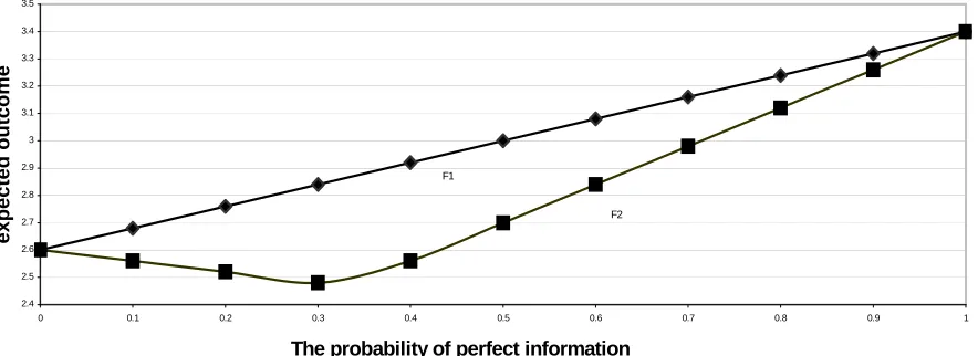
The comparison between those two scenarios is dem-onstrated in Figure1:
By observing the aforementioned example it can be concluded that, when a new (improved) information sys-tem is syssys-tematically more informative than the current information system two important goals are achieved:
1) “Decision situation independence” -The ability to
implement the information system step by step and to improve the level of informativeness is guaranteed.
2) “Life-cycle independence” -The ability to
imple-ment the information system without interfering the users (the decision makers) and while existing expected out-comes are guaranteed (without the necessity to start training and testing processes).
5. Towards Assessing the Systematic
Informativeness Ratio between Noisy
Information Structures – the Dominancy
of Trace
A characteristic of F is that its diagonal elements are
(weakly) dominant (in accordance with Definition 4). From Theorem 3 it can be shown that this characteristic is a necessary condition for existence of the systematic informativeness ratio between I and Q:
Theorem 334
Let I (the identity matrix), and Q be two information structures. S{S1,..,Sn} is the common set of states of nature, and Y{Y1,..,Yn} is their same set of signals
they produce.
1 i,i j,i
S
I Q i,i ,..,n, Q Q i j (The diagonal el- ements are weakly dominant in each and every column).
[image:9.595.309.537.112.303.2]This theorem implies that the dominancy of the di-agonal elements in each and every column of an infor-
Table 2. Expected compensation in various levels of prob. for perfect information (1st scenario)
Expected
compen-sation The
prob-ability to receive F1 The probability
to receive I. Characteristics
of the Decision situation 2.6 1 0 2.76 0.8 0.2 2.92 0.6 0.4 3.08 0.4 0.6 3.24 0.2 0.8 3.4 0 1 A-priory probabilities: (0.2,0.6,0.2) Perfect information 1 0 0 0 1 0 0 0 1 Partial information 1 0 0 0 0 1 0 0 1
Table 3. Expected compensation in various levels of prob-ability of perfect inf. (2nd scenario)
Expected
compen-sation The
prob-ability to receive F2 The probability
to receive I
Characteristics of the Decision
situation 2.6 1 0 2.52 0.8 0.2 2.4666 0.666 (2/3) 0.333 (1/3) 2.56 0.6 0.4 2.84 0.4 0.6 3.12 0.2 0.8 3.4 0 1 A-priory probabilities: (0.2,0.6, 0.2) Perfect information 1 0 0 0 1 0 0 0 1 Partial information 0 1 0 0 0 1 0 0 1
mation structure is a necessary condition for the exis-tence of a systematic informativeness ratio between the identity information structure (which represents complete information) and the non-identity information structure. This casts a preliminary condition for the existence of the informativeness ratio.
The following example demonstrates, by using Theo-rem 3, that the systematic informativeness ratio is not always transitive.
1
1 0 0
1 0 0
0 0 1
F , 2
1 0 0
0 1 0
0 1 0
[image:9.595.58.272.150.244.2]2.4 2.5 2.6 2.7 2.8 2.9 3 3.1 3.2 3.3 3.4 3.5
0 0.1 0.2 0.3 0.4 0.5 0.6 0.7 0.8 0.9 1
The probability of perfect information
ex
pected outcom
e
F1
[image:10.595.81.523.95.256.2]F2
Figure 1. A comparison between the two scenarios
1 1
1 0 0
0 25 0 75 0 25 0 1 0
0 0 1
1 0 0 1 0 0
0 75 1 0 0 0 75 0 25 0
0 0 1 0 0 1
Q . * I . * F . *
. * . .
2 1 2
1 0 0
* 0 4 0 6 0 75 0 25 0
0 0 1
Q Q . * I . * F . . *
1 0 0 1 0 0
0 4 0 1 0 0 6 0 1 0
0 0 1 0 1 0
1 0 0 1 0 0 1 0 0
0 75 0 25 0 0 1 0 0 75 0 25 0
0 0 1 0 0 6 0 4 0 0 6 0 4
. * . *
. . * . .
. . . .
Since F1F, from Theorem 2 it is concluded that
1
Q I
S
. Moreover, since F2F, from Lemma 1 it is
concluded thatQ1 Q2
S
. However, from Theorem 3, it is
concluded that sinceQ23,2Q22,2, I is not systematically
more informative than Q2.
Since the systematic informativeness ratio is not al-ways transitive, when there is a multi stage implementa-tion and improvement program during the life-cycle of a decision-support information system and the informa-tiveness ratio of this information system can be improved systematically, the preservation of systematically infor-mativeness ratio is not automatically guaranteed during the whole life-cycle of information system. Hence, the importance of a long-range perspective arises. This can be achieved in one of two ways, depending on the ability to guarantee whether the last version of information structure can be systematically more informative than any previous version, or only superior to its predecessor version:
When the systematic informativeness ratio can be ob-tained between each and every two sequential versions of an information system during its lifecycle, then a long- range plan of the versioning mechanism is required. This could guarantee that the latest version of an information system will be systematically more informative than any of the previous versions. Moreover, it will guarantee a growth (or at least stability) in expected outcomes during the lifecycle of the decision support system, without alerting the decision makers. Hence, implementation and training processes between versions of the information system become less critical.
6. A Summary and Conclusions
This paper analytically examines and identifies the sys-tematic informativeness ratio between two information structures. The methodological approach presented here may lead to a better understanding of the performances of decision support information systems during their life-cycle.
This approach may explain, normatively, the pheno- menon of “leaks of productivity”. In other words it may explain the decrease in productivity of information sys-tems, after they have been improved or upgraded. This degradation in the expected outcomes can be explained by the inability of the users to adapt immediately to new decision rules.
It can be assumed that the usage of the methodology that was presented in this paper to improve or replace information structure with systematically more informa-tive versions of information structures over time may facilitate the achievement of the following major targets:
1) Increase the expected payoffs over time.
2) Reduce the risk of failure of new information sys-tems as well as new versions of information syssys-tems.
3) Reduce the need to cope with complicated and ex-pensive training processes during the implementation stages of information systems (as well as the implemen-tation of new versions of the systems). Moreover, some-times this process can be completely skipped during the installation of a new version of an information system.
The paper analyzes the conditions for the existence of a systematic informativeness ratio between I -the identity information structure which represents complete infor-mation, and another information structure. In the case of non-noisy information structures the necessarily and suf-ficient conditions for existence of the systematic
infor-mativeness ratio between I and a second information
structure are set and proved comprehensively. As a result, some necessary and sufficient conditions are set, proved and demonstrated for the noisy information environment as well.
Further research can be carried out in some directions: 1) Exploration of additional analytical conditions for the existence of the systematic informativeness ratio be-tween I, the identity information structure and noisy in-formation structures.
2) Classification of cases where the systematic infor-mativeness ratio inheritably exists by using the condi-tions those are set so far.
3) Devising empirical methods to examine the impact of using the principle of developing decision support information systems is systematically more informative over time, on the performance of decision-makers, as well as on their perceived satisfaction from using those systems.
4) Designing empirical studies (experiments, case studies and surveys) to validate the theoretical analysis
provided here.
REFERENCES
[1] C. E. Shannon and W. Weaver, “The mathematical theory of communication,” University of Illinois Press, Urbana, Illinois, 1949.
[2] H. Raiffa, “Decision analysis,” Reading, Addison-Wesley, Massachusetts, 1968.
[3] G. A. Feltham, “The value of information,” The Ac-counting Review, Vol. 43, No. 4, pp. 684–696, 1968. [4] J. Marschak, “Economic of information systems,” Journal
of the American Statistician Association, Vol. 66, pp. 192–219, 1971.
[5] C. B. McGuire and R. Radner, (editors), “Decision and organization (ch. 5),” University of Minnesota Press, 2nd edition, Minneapolis, Minnesota, 1986.
[6] H. A. Simon, “The new science of management deci-sions,” Harper and Row, New-York, 1960.
[7] A. Rubinstein, “Modeling bounded rationality,” MIT. Press, Cambridge, Massachusetts, 1998.
[8] N. Ahituv and Y. Wand, “Comparative evaluation of information under two business objectives,” Decision Sci-ences, Vol. 15, No. 1, pp. 31–51, 1984.
[9] N. Ahituv, “A comparison of information structure for a ‘Rigid Decision Rule’ case,” Decision Science, Vol. 12, No. 3, pp. 399–416, 1981.
[10] N. Ahituv, “Describing the information system life cycle as an adjustment process between information and deci-sions,” International Journal of Policy Analysis and In-formation Systems, Vol. 6, No. 2, pp. 133–145, 1982. [11] G. Ariav and M. J. Ginzberg, “DSS design: A systemic
view of decision support,” Communications of the ACM, Vol. 28, No. 10, pp. 1045–1052, 1985.
[12] E. Brynjolfsson, “The productivity paradox of informa-tion technology,” Communicainforma-tions of the ACM, Vol. 36, No. 12, pp. 67–77, 1993.
[13] E. Brynjolfsson, “Paradox lost,” CIO, Vol. 7, No. 14, pp. 26–28, 1994.
[14] E. Brynjolfsson and L. M. Hitt, “Beyond the productivity paradox,” Communications of the ACM, Vol. 41, No. 8, pp. 49–55, 1998.
[15] N. Ahituv and G. Greenstein, “Systems inaccessibility and the productivity paradox,” European Journal of Op-erational Research, Vol. 161, pp. 505–524, 2005.
[16] M. C. Anderson, R. D. Banker, and S. Ravindran, “The new productivity paradox,” Communications of the ACM, Vol. 46, No. 3, pp. 91–94, 2003.
[17] N. Ahituv and Y. Elovici, “Evaluating the performance of an application running on a distributed system,” Journal of the Operational Research Society, Vol. 52, pp. 916-927, 2001.
pp. 75–97, 2003.
[19] L. Aronovich and I. Spiegler, “CM-tree: A dynamic clus- tered index for similarity search in metric databases,” Data & Knowledge Engineering, Vol. 3, pp. 919–946, 2007.
[20] N. Ahituv and B. Ronen, “Orthogonal information struc-ture—a model to evaluate the information provided by a second opinion,” Decision Sciences, Vol. 19, No. 2, pp. 255–268, 1988.
[21] Z. Safra and E. Sulganik, “On the nonexistence of black-well’s theorem-type, results with general preference rela-tions,” Journal of Risk and Uncertainty, Vol. 10, pp. 187–201, 1995.
[22] E. Sulganik and I. Zilcha, “The value of information the case of signal dependent opportunity sets,” Journal of Ec- onomic Dynamics and Control, Vol. 21, pp. 1615–1625, 1997.
[23] B. Ronen and Y. Spector, “Theory and methodology
evaluating sampling strategy under two criteria,” Euro-pean Journal of Operational Research, Vol. 80, pp. 59–67, 1995.
[24] N. Carmi and B. Ronen, “An empirical application of the information-structures model: The postal authority case,” European Journal of Operational Research, Vol. 92, pp. 615–627, 1996.
[25] N. Margaliot, “Selecting a quality control attribute sample: An information-economics method,” Annals of Opera-tions Research, Vol. 91, pp. 83–104, 1999.
[26] B. Ronen, “An information-economics approach to qual-ity control attribute sampling,” European Journal of Op-erational Research, Vol. 73, pp. 430–442, 1994.
Appendix
Theorem 1:Let Q1 and Q2 be two information structures operating
on the same set of states of nature S = {S1,…,Sn}, and
producing the same set of signals Y = {Y1,…,Ym}. Then
2 1 Q
Q S
p,0 p1, p*Q1(1p)*Q2Q2First, Lemma 1.1 is proven.
Lemma 1.1:
Let Q1and Q2 be two information structures
de-scribing information systems. Let S = {S1,…,Sn} be their
set of the states of nature of Q1 and Q2 . Let
Y={Y1,…,Ym} be their set of signals. Then for any given
decision situation described by (a matrix of a-priori
probabilities of states of nature), U (a matrix of utilities or compensations), A (a set of decisions), where
Dpure -max(Q )2
is the set of optimal decision rules whenQ2 is used, there exists >0, such that if 0<p, and Dp is
an optimal decision rule of the Information structure
1 1 2
p* Q ( p)* Q
Then Dp
Dpure -max(Q )2
.Proof (of Lemma 1.1):
1) It can be assumed that every optimal decision rule is a convex combination of pure decision rules [10]. So we try to find the optimal decision rule of
1 1 2
p* Q ( p)* Q in the set of the optimal pure deci-sion rules of Q2, Dp
Dpure -max(Q )2
.2) Let k be the number of possible decisions in this
given decision situation. This means that there are
k
mpure decision rules, denoted D ,..,D1 km.
Let
Dpure
the full set of the possible pure decision rules for this given decision situation3) If
Dpure -max(Q )2
Dpure
, that means that every pure decision rule is an optimal decision rule it is obvious that Dp
Dpure -max(Q )2
.4) So, assume that
Dpure -max(Q )2
Dpure
.
5) Hence:
Dpure
\ Dpure -max(Q )2
6) Let’s calculate for every pure strategy Di the fol-lowing values: V1itrace(Π*Q * D * U),1 i
2i * 2 i
V trace(Π Q * D * U)
7) trace(Π*(p* Q (1 1 p)* Q )* D * U))2 i
8) 1
2
1
i
i
p* trace(Π* Q * D * U)) ( p)* (trace(Π* Q * D * U))
9) p* V1i (1 p)* V2i
10) Let’s define in this specific decision situation:
1max
1iD
V Max V - The (optimal) expected value when using the information structure Q1.
1
1max 2
i
Di Dpure- (Q )
V Max V
- The (optimal) expected
value when using the information structure Q1, when the
set of decision rule is limited to the optimal set of pure decision rules when using the information structure Q2.
2 max
2max 2
i
Di Dpure- (Q )
V Max V
- The (optimal) expected
value when using the information structure Q2.
2
2max 2
i
Di Dpure- (Q )
V Max V
- The (optimal) expected
value when using the information structure Q2, when the
set of decision rule is limited to the non-optimal set of pure decision rules when using the information structure
Q2.
11) According to expression (4)
Dpure- (Q )
Dpure
2 max
Hence:ΔV2(V2max-V2)0
12) Moreover: ΔV1(V1max-V1)0
13) Let’s examine for Di
Dpure
\Dpure-max(Q2)
whenit is not an optimal decision rule of p*Q1+(1-p)*Q2. We
try to identify a small value of p that will always give
max 2 1
2
1 (1 p)*V p*V (1 p)*V
p*Vi i . In fact, the
purpose is to find an “environment” of Q2 where an
opti-mal decision rule of Q2 is also an optimal decision rule of p*Q1+(1-p)*Q2.
14) From (9) it is concludes that
2 1
2
1 (1 p)*V p*V max (1 p)*V
p*V i i
15) Let’s examine weather exists:
max max
1 1 2 1 1 2
p* V ( p)* V p* V ( p)* V
16)
2 2 1
2 2 2 2 1
1max max max
V ) V V p*(
-V V -V V p* -V V p*
Δ Δ
Δ
2 1
2
0
V V
V p
Δ Δ
Δ
That’s according to (10), (11) 0
0 1 2
2 0
1 V , V V
V , Δ Δ Δ
Δ
17) Let’s pick: 0 1
2 1
2
V V
V
ε
Δ Δ
Δ
18) And in this environment (for every 0p) at
least one optimal decision rule of Q2 is an optimal
deci-sion rule of p*Q1+(1-p)* Q2
Q.E.D (Lemma 1.1) Proof (of the theorem itself):
First direction: assume that for every decision situa-tion:
1) DMax(trace(D (QΠ)}, trace(Π))*Q*D *U)
2 D
Q 1 2
max {
Q2 2
*D*U *Q