Evaluation of Multiusers’ Interference on Radiolocation
in CDMA Cellular Networks
A. J. Bamisaye, M. O. Kolawole, V. S. A. Adeloye
Department of Electrical and Electronics Engineering, The Federal University of Technology, Akure, Nigeria E-mail: {ayobamisaye,kolawolm, vadeloye}@yahoo.com
Received October 17, 2009; revised November 15, 2009; accepted December 16, 2009
Abstract
Radiolocation has been previously studied for CDMA networks, the effect of Multiple Access Interference has been ignored. In this paper we investigate the problem of Radiolocation in the presence of Multiple Ac-cess Interference. An extensive simulation technique was developed, which measures the error in location estimation for different network and user configurations. We include the effects of lognormal shadow and Rayleigh fading. Results that illustrate the effects of varying shadowing losses, number of base stations in-volved in position location, early-late discriminator offset and cell sizes in conjunction with the varying number of users per cell on the accuracy of radiolocation estimation was presented.
Keywords:Code Division Multiple Access, Radiolocation, Multiple Access Interference, Base Station, Mobile Station.
1. Introduction
Radiolocation involves: a) identifying the base station (BS) that would participate in the process of subscriber location by selecting a set of BSs within the coverage area that receives intelligible levels of signal from the mobile station (MS) under consideration. b) estimating one-dimensional position which involves each BS, par-ticipating in the process, independently producing an estimate of the subscriber location based on its meas-urements; c) location estimation, that is, estimates from all the participating BSs are used by position location algorithms to produce an accurate estimate of the sub-scriber location within the coverage area. But, the esti-mates produced are not always very accurate. The major sources of error in subscriber location systems are: tipath propagation, non-line-of-sight (NLOS), and mul-tiple access interference (MAI). In the case of multipath propagation, accuracy is greatly affected when the re-flected rays arrive within a very small period of the first arriving ray. Case is even more worsened when the power of reflected rays is more than the first arriving ray [1]. Several methods have been developed to mitigate the effects of multipath on radiolocation. Typically propaga-tion in wireless communicapropaga-tions accrues up to an aver-age of 400-700m [2,3] and biases the estimations. By
using the a prior information about range error statistics,
range estimations made over a period of time and
rupted by NLOS errors can be adjusted to near their cor-rect values. An alternative approach is to reduce the weights of the BSs prone to NLOS reception while esti-mating location using position location algorithms [4,5]. Co-channel interference is a problem faced by all the
cellular systems. In Code Division Multiple Access
(CDMA) networks, users share the same frequency band, but use unique pseudo-noise (PN) codes. Near far effects in CDMA networks are the biggest source of errors in position estimation. Multiple cellular users who are using the same frequency allocation at the same time cause MAI: it greatly affects the performance of Time of Arri-val (ToA) estimation of CDMA systems. In CDMA cel-lular systems, the MSs are power controlled to combat the near-far effect. Thus, for a CDMA network, time based approach is the most promising technique. This paper investigates the effect of MAI and the accuracy of Radiolocation in CDMA cellular network.
This paper models the intracellular and intercellular multiple access interference (MAI) in Section 2, simula-tion results are presented in Secsimula-tion 3, and finally in Sec-tion 4, the conclusion drawn from the study is summa-rised.
2. System Model
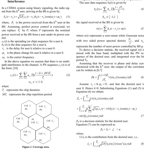
other than the intended user, act as interfering signals, thereby giving rise to multiple access interference. Figure 1 represents such a situation.
With reference to Figure 1, the coverage area comprises
of cells, , and . These cells have
,
i
C Cj, Cp
i
n nj users respectively. The BS’s i,
j ,k ,.... and p exercise power control over the users they
serve. Let Ai, Aj , Ak....and Ap denote their areas. Only few cells have been considered for simplicity of explanation.
, and
k
n Cp
2.1. Modeling Intracellular Multiple Access Interference
In a CDMA system using binary signaling, the radio
sig-nal from the kth user, arriving at the BS is given by:
( ) 2 ( ) ( ) cos(
k k k k k k k c k
S t P c t b t t ) (1)
where, is the power received from the kth user at the
BS. Assuming, perfect power control is exercised, we
can replace by P, where P represents the nominal
power received at the BS from a user under its power con-trol.
k P
k P
ck (t) is the spreading (or chip) sequence for a user k.
bk (t) is the data sequence for a user k.
k
is the delay for user k relative to a user 0.
k
is the phase change for user k relative to a user 0.
k
is the carrier frequency.
In the above equation we assume that there is no
multi-path interference in the channel. A PN sequence ck (t) is of
the form: [10] 1
, 0
( )
( ) M ( c)
k k i
j i c
t i jM T
c t a
T
(2), { 1.1}
k i a
where
c
T represents the chip duration.
c
MT represents the chip repetition period.
Cell Ci
i
BS
Cell Cn
n
BS
k
BS
Cell Ck
Cell Cj
j
BS
Cell Cp
p
BS
Cell Cl
l
BS
Cell Cm
m
[image:2.595.51.537.221.725.2]BS
Figure 1. Coverage area.
Π represents the unit pulse function given by
1 0 t 1
( )t
0 otherwise
(3)
i is an index to denote a particular chip within a PN
Tb = GTc
where G represents the factor or gain of the
cycle. For data sequence bk(t), Tb is the bit period
such that
spreading
CDMA system. It is not necessary that the gain G of a
CDMA system be equal to M. In case they are same, a
PN sequence would be repeated for every bit period Tb.
The user data sequence bk(t) is given by
,
( ) ( b)
k k i
j b
t jT
b t b
T
(4)
, 1,1
k i b
the signal received at the BS is given by
(5)
where n(t) esents a zero-mean white Gaussian noise
0
( ) k( k) ( )
k
r t S t n t
np repr
with two sided power spectral density
2
o
N , and n
represents the number of users power contro BS
To derive a decision statistic, the received signal r(t) is
p
lled by p.
m
g that the receiver is phase and delay syn-ch
ixed with the base band, multiplied with the PN se-quence of the desired user, and integrated over the bit period Tb.
Assumin
ronized with the kth user, the output of the correlator
can be written as [6,7]
(j 1)
( ) ( ) cos( )
b
k c
b T
Zk r t c t
jT
t dt (6)Assume
0,
k k 0
Substi
, and that the desired user is
user 0. Hen tuting Equations (1) and (5) in
Equation (6) we obtain T
ce k=0.
0 0[ ( ) ( ) cos(0 )
b
c
Z r t c t t dt
t
1
0
[( 2 ( ) ( ) cos( )
0
p n b
k k k k c k
k
T
p c t k b t t
t
0
( )] ( ) cos( c )
n t c t t dt
(7)
Z0 is a decision statistic for the desired user. Equation (7) can be expressed as
Z0 = I0 + + η where
he contribution from the desired user, i.e.,
1) I0 is t
2 2
0 0 2 0( ) ( ) cos ( )
b
k k c
T
P b t c t t dt
t
(8)As Hence
2
{ 1,1}, 1
k k
c c
0
I reduces to
0 0 2 0( ) b
P
I b t T (9)
2)
mati
represents the contribution of MAI and is the
sum on of np1 terms, Ik, where
2 ( ) ( )
k k k k k k
I p c t b t
0
( ct k) ( ) cosc t
cos (ct dt) (10)
1 0 p n k k I
(11)3) η represents the contribution of noise and is given by
(12)
To determine the variance and mean of η
t (13)
Variance
0
0
t ( ) ( ) cos( )]
b
c
T
n t c t t dt
0
0 c
t
[ ] b [ ( ) ( ) cos( )] 0
T
E E n t c t t d
2
2 2 2
0
[( ) ] [ ]
[ ( ) ( ) cos( ) ( ) cos( ) ]
0 0
b b
c c
E E
T
E n t n c t t dt d
t T
Now, 0) ( ) N ( )
t n t
[ (
2
E n
2 0
0( ) cos( ) ( ) cos(0 ) ( )
0 0 2
b b
c c
T T N c c t t t dt d t
02 0 2( ) cos (2 )
0 2
b
c
T N
c t t dt
t
02( ) 1
c t Hence
2 0(1 cos(2 ))
0 0 4
b b
c
T T N
t dt t
2 0 4 b N T (14)
Assuming a large number of interferes, by virtue of the
central limit theorem (CLT), the distribution of can
be approximated by a zero-mean Gaussian distribution
[4,7,8] with variance 2
given by [7]
1 2 2 1 6 p n
c k k
GT P
(15)Let,
Assuming that the MAI and noise are independent
proc-, the variance of
(16)
esses can be written as
2 2 2
(17) 1
2
1 0
n
c k
GT P N T
6
p
k b (18)
2.2. Modeling Intercellular Mult
ed by
the at epresented by
4
iple Access Interference
Expression for the intercellular interference caus
users of cell Ci BS j,r Iij can
be derived. Let the h l ponent e
p
pat oss ex
y
be m. Let th
fading on path from this user to cell Ci be Rayleigh
distributed, and re resented b xi. Similarly, let the
fading on the path from this user to cell Cj be Rayleigh
distributed, and represented by xj. The average of 2
i
x is the log-normal fading on the path from this user to cell
i, i.e, [ 2 10i/10
i i
E x , where
i
is the decibel
at-tenuation due to shadowing, and is a Gaussian random
variable with zero-mean and standard deviation s
[9,10]. Similarly the average of 2
j
x is the log-normal
fading on the path from this user to cell. j Let
k
P be the
nominal power received at BS i from user ni.It is
as-sumed that the power control m hanism overcomes both the large scale path loss and shadow fadin How-ever, it does not overcome fast fluctuation of signal power due to Rayleigh fading [8,11]. As BS i exercises a power control over the MS, the actual transmission
power Paciof the MS would be
/10
[ ( , ) 10i ]
i
m ac i i
P P r x y (19)
where (x, y) is the distance
ec g. s i r quent
of the MS from BS i.
Conse y, assuming uniform user
the relative average interference
l density in the cell,
ij
I at cell C jcaused by
s
all the u ers in cell Ciis given by [9]
/10
2
1 ( , )10
[ ( , )] ( , ) i m i i ij m i i i
n r x y
j
I E dA x y
c
A r x y
x
(20)by using iterated expectations,
2 2
10 10
[10 . ] [ [10 . , ]]
i i
j j i j
E x E E x
2 10
[ [10 . ]]
i
i j j i j
E E x
Given i and j
2
[ j i, j]]
E x
10
10 i
Thus,
( ) 2
10
[10 . ]
i
j
E x
[10 10 ]
i j
E
Let X i j Thus, X is
o 2
a Gaussian variable of zero-mean and variance
equal t 2
S
2 10
[10 . ]i [ x]
j
E x E e
2 2
4
i S
x x
2 10
2
[10 . ]
4
j
e e
E x dx
S
2
( ) 2 10
[10 . ]i s
j
E x e
(21)
where = In(10)/10 =.2303. Substituting the result
back in 0) we obtain (2
2
( ) 1 ( , ) ( , )
( , )
m i
i j
s
m
i i
ij
n r x y
I e
dAx y (22)c
A r x y
If denotes the voic
equation becomes
e activity factor, then the above
2
( ) 1 ( , ) ( , )
( , )
s
m
i i
ij m
i
i j
n r x y
I e
dA x yc
A r x y
Let ij
(23)
K denote inter-cell interference factor due to a
user in cell i at BS j. Hence,
ij ij
i K
n
I (24)
2
(s) 1 ( , ) ( , )
( , )
m i
m i
i j
r x y
e dA x y
c
A r x y
(25)In our model Kii
0
ij
is zer ). It
o at cel
wise (i.e, portant to point out the
im-portance
l ii, but not zero
other-ij
K of
is im
K . Kij gives the interference at BS j
caused by a sin user in cell i. Thus, if the total number
of users in cel were to change, the new interference
levels can ned by simply taking a product of ij
gle l i
obtai
be K
and the numb f rs. This simplifies our calculations
as the interference need not be recalculated for the new number of users. Thus, using Equation (23) we can compute relative average intercellular interference uniform user distribution. Thus, for an uniform user dis-tribution, we can write the total intercellular interference at BS j due to users in cell i a
ij i ij
er o use
for
I n K (26) It should be noted that the above interference
calcula-tions are assuming nominal power as unity. If P is the
nominal power from a power controlled user received at
home BS, then Equation (26) would be modified as
ij i ij
I p n K (27) Equation (27) gives the total intercellular interference at cell Cj due to users in cell Ci.
3. Simulation and Results
lat with the following set of
d parameters:
selected. Hence, Rc =
system is 128. Hence Simu ion was carried out
fixe
A chip rate of 1.2288MHz was 1.2288 Mcps; gain of the CDMA
G=128; Path loss exponent for mobile communications is
4 [11]. Hence, m=4;As we are restricting the interference
from the first tier of interferer’s, number of cells in the
coverage area is 7. Hence, NBS = 7; Nominal power of
MS, Pk = 1; Speed of radio signal, C = 3x10⁸ m/s;
Ther-mal noise, 0 108
2
N ; User distribution per cell is
uni-form and every cell has same number of users N. The
variable sets of parameters include:
a) N: Num er of users per cell;
b)
b
s
: T d deviation of shadowing losses in
every cell; c)
he standar
BS
N : Number of BS’s participating in
radioloca-tion;
d) : DLL(delay-locked loop) resolution.
e) R: Radius of the cells.
g th
ize of cells on
d to study the combined
1)
We studied the effects of varying shadow losses,
varyin e number of BS’s participating in radiolocation,
varying the DLL resolution and varying the s
the ccuracy of estimation. a
3.1. Effect of Varying Shadowing Losses on the Accuracy of Radiolocation
This experiment was conducte
effect of varying shadowing losses and the number of users per cell on the error in radiolocation.
Set 1
8, number of BSs participating in
radio-any computer system that supports the
location = 3, radius of the cell = 1500m. and integration period, Tint = 128Tc. Generate a cell site BS database for 7 cells of radius 1500m each, using
graphical user interface, GUI. Set value
of sto 6dB.
2) For the given value of s compute the interference
matrix Fij.
3) The number of user is vary per cell from 1 to 100, in steps of 10, and estimate the error in position estima-tio
il , set
n
4) Sim arly s=8dB and 10dB, and go to Step 2.
re carried out. The final results are an
av-er o
ou
random locations were chosen within the central cell, and estimations we
evident that introdu the third estimator ha gnificant
impact on the estimation accuracy and
2) There no si ant im ent in timation
accuracy when the nu er of B increase 3 to 4:
The mean radiolo error es by hen we
increase the number of BS’s to ow , there is
lower accuracy re-qu
for esti-ating the TOA of the received signal. The accuracy of
ely
the D ined
by th study the effect of variation of ∆ on
e accuracy of estimation, we have performed experiments age of the results btained at the 50 locations. Similar
procedure is carried t for the remaining set of experi-ments.
The plot in Figure 2 shows the variation of error in
radiolocation with number of users per cell and s. The
mean value of the radiolocation error, tabulated below is determined by taking an average of all the points plotted in the Figure 2. When the number of users is varied from 1 to 100, and other conditions remaining the same, the mini-mum, maximum and mean values of the observed errors are tabulated in Table 1. The mean error in two-dimen-sional position estimation remains almost constant when
s
is increased from 8 dB to 10 dB.
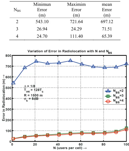
3.2. Effect of Varying the Number of Participat-ing BS’s on the Accuracy of Radiolocation
e used 2,3 and 4 BS’s to estimate th
W e subscriber location
.
1) n
under the above heading. The results are plotted in Figure 3 It was observed that:
Accuracy improves drastically if we use more tha two BS’s for estimation: The accuracy of estimation im-proves to 71.51m from 697.12m when we employ 3 BS’s to estimate the subscriber location instead of 2. Thus, it is very
[image:5.595.61.283.400.577.2]Figure 2. Variation of radiolocation error with N and s.
Table 1. Min and max error in radiolocation for different values of s
σs Minimun Maximim Error mean
(dB) Error (m) (m) Error (m)
6 26.30 364.33 122.40 8 25.83 122.30 71.51
10 25.85 96.92 75.40
cing s a si
is gnific provem the es
mb
cation improvS’s is 6m wd from
4. This sh s that
no effect obtained when we increase the number of BS’s from 3 to 4. For applications with
irements, 3 BS’s would be sufficient for radiolocation. Table 2, derived from Figure 3, outlines the minimum, maximum and mean values of estimation errors for various values of NBS as the number of users per cell is varied from 1 to 100, other conditions remaining same.
3.3. Effect of Varying the Early-Late Discriminator Offset on the Accuracy of Radiolocation
For our work we have used a non-coherent DLL m
estimating the TOA using a DLL depends on how clos LL can track the incoming signal, and this is def
e parameter ∆. To
th
with ∆= 1 1,
2 4 and
1
8.The results of the experiment are
plotted in Figure 4.
Table 2. Min and max error in radiolocation for different val-ues of NBS.
NBS
Minim Erro (m
Maximim mean
un r )
Error (m)
Error (m) 2 543.10 721.64 697.12
3 26.94 24.29 71.51
[image:5.595.313.532.442.699.2]4 24.70 111.40 65.39
[image:5.595.86.257.641.714.2]la
would be inefficient for such cases.
igure 4, the accuracy of estimation, falls as the
number of ce is because of the
degradation o R (sig noise) w ing
num-ber of users p ll.
[image:6.595.65.278.80.258.2]3.4. E ect of Varying the Cell Size e Accuracy of Radiolocation
Figure 4. Variation of radiolocation error with N and ∆.
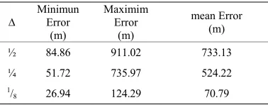
Table 3, derived from Figure 4, outlines minimum and
maximum values of errors for different values of ∆ as the
number of users per cell are increased from 1 to 100, other conditions remaining same. The mean radiolocation error reduces to 524.22m and 70.79m from 733.13m and
524.22m respectively when ∆ is reduced from 1
2 to
1 4
and from 1
4 to
1
8. But, the lowest value of ∆ is limited
by
a) In practice, the locally generated PN sequence will have to be phase delayed to generate the early and late PN sequences. As per IS-95 standards, one chip period corre-sponds to 813.80 nSec. Thus, if we were to deploy a tracki g
loo n
ca ility on the hardware will be
a til
n
PN sequence is delayed by T . If ∆ = 1/k, there are k po-
o search through before it can lock to the sub-n
p with ∆=1/16, the requirement on the timing resolutio
pab
∆t = Tc × ∆= 813.08nSec/16=50.8175nSec
Implementing such high precision tracking loops is both challenging and expensive.
b) If the DLL employ’s a serial search technique, it
will have to search through all potential code del ys un the correct delay is identified. Suppose, the i coming
c
tential delay values between 0 and Tc that the DLL will have t
[image:6.595.76.265.641.715.2]scriber signal. Thus, the size of the set of potential de-
Table 3. Min and max error in radiolocation for different values of ∆.
∆
Minimun Error
(m)
Maximim Error
(m)
mean Error (m)
½ 84.86 911.02 733.13
¼ 51.72 735.97 524.22
1/
8 26.94 124.29 70.79
ys increases as the value of ∆ decreases. The bigger
the set of potential delays, the longer it will take for the tracking loop to achieve a lock. The situation becomes more complicated, if we are also estimating the velocity of the subscriber. The set of potential delays, soon trans-forms into a two-dimensional matrix defining the set of potential delays and velocities. A serial search technique
Also, accuracy falls as number of users per cell increases. As seen in F
users per
f SN ll increases. This nal-to- ith increas er ce
ff on th
All the earlier experiments were carried out with cells, each of radius 1500m. In this case, we simulated coverage areas with cell radii 100m and 500m. Simulations were
carried out under the following conditions: 1
8;σs =
8dB; and number of BSs involved in radiolocation = 3. The number of users is varied from 1 to 100 in steps of 10.
The results were then compared wi tth he results of the
ex
is better with smaller cells. 100m,
ca-tion
orks
e ps
ultiple ac
ave studied the effect f MAI in conjunction with varying shadowing
envi-racking capability of the DLL, participating in radiolocation, and periment carried out under identical situation but using cells of 1500m radius. The results indicate that under per-fect power control, the degradation in SNR (signal-to-noise) with number of users is independent of the cell size; and the accuracy of estimation
For the experiment conducted with cells of radii 500m and 1500m, it is found that accuracy of radiolo
is best for cells of radius 100.
4. Conclusions
Our study has investigated the possibility of accurate
subscriber location in CDMA cellular netw in the
presence of multiple access interference. Earlier works have ignored the effect of non-orthogonality of th
eudo-noise codes on the estimation accuracy. They usually consider the case of a single MS with no inter-ferers, which is not a practical assumption. In our work, we have studied the effect of number of interferers on the accuracy of estimation by varying the number of users in every cell from 1 to 100. To study the effects of m
cess interference on the accuracy of estimation, we have assumed the presence of a line-of-sight component between the MS and the BS. We h
o
ronments, varying t ng number of BSs i
interfer-] M. Hata and T. Nagatsu, “Mobile location using sig-easurements in a cellular system,” IEEE
ehicle Technology, Vol. 29, pp. 245–
Transactions on
90.
ference, pp. 919–923, 1997.
ence is present.
5. References
[1] R. Ilts, “Joint estimation of PN code delay and multi-path using extended kalman filter,” IEEE Transactions on Communications, Vol. 38, pp. 1677–1685, October 1990.
[2] M. Silventoinen and T. Rantalainen, “Mobile station emergency locating in GSM,” Proceeding of IEEE In-ternational Conference on Wireless Communications, pp. 232–38, 1996.
[3] M. Wyile and J. Holtzman, “The non line of sight problem in mobile location estimation,” Proceedings of IEEE ICUPC, pp. 827–831, 1996.
[4] J. Caffery, Jr, and G. Stuber, “Subscriber location in CDMA cellular networks,” IEEE transactions vehicle technology, Vol. 47 No. 2, pp. 406–15, May 1998. [5
nal strength m Transactions V 251, May 1980.
[6] R. K Morrow, Jr., and J. S. Lehnert, “Bit-to-bit error dependence in slotted DS/SSMA packet systems with random signature sequences,” IEEE
Communications, Vol. 37, No. 10, October 1989. [7] T. S. Rappaport, “Wireless communications principles
& practice,” IEEE Press, New York, Prentice-Hall, 2002.
[8] A. J. Bamisaye and M. O. Kolawole, “Evaluation of downlink performance of a multiple-cell, rake receiver assisted CDMA mobile system,” Journal of Wireless Sensor Network, 2009.
[9] R. G. Akl, M. V. Hegde, A. Chandra, and P. S. Min, “CCAP: CDMA capacity allocation and planning,” Tech Republic, Washington University, April 1998. [10] W. C. Y. Lee, “Mobile cellular telecommunications,
analog and digital systems,” 2nd Edtion, McGraw-Hill, Inc, 19