Controlling Characteristics of the Slot Wave by Virtual Capacity Setting:LIP Solving Slot Allocation Based on Data Splitting Method
ZhiJian Ye1* Wenpeng Zhai 2 XinXin Zheng3 Shihao Huang4
1 College of Air Traffic Management, Civil Aviation University of China, Tianjin300300, China;
2 College of Air Traffic Management, Civil Aviation University of China, Tianjin300300, China;
3 College of Cabin attendant, Civil Aviation University of China, Tianjin300300, China;
4 College of Air Traffic Management, Civil Aviation University of China, Tianjin300300, China;
Correspondence: ZhiJian Ye. [email protected]; +86-13022226938
Abstract:Management of demand and capacity for airport operation is important. The effect of capacity setting on slot adjustment, maximum adjustment and flight delay has been extensively investigated and discussed in previous slot adjustment models. But its effect on characteristics of flight waves has not been studied deeply. At present, in order to resolve the problem that Linear Integer Programming (LIP) is limited in slot allocation due to its fast dimension growth and large memory consumption, the general practice is to optimize the slot application according to data-splitting technology. However, the relationship among data splitting method, capacity setting and characteristics of slot wave has not been investigated in detail, which limits the application of LIP in slot allocation. Through the detailed analysis and testing, we found that the waveform and amplitude of slot wave can be controlled and designed by appropriate virtual capacity settings, while the number of capacity constraints and the computing time is reduced by adopting appropriate data feeding method. Our research also provides clues for further research on the construction of the flight waves for airlines operating at specific airports in order to establish direct or indirect connectivity, and increase hit rate by using our approaches.
Keywords:Slot Allocation; Characteristics of Slot Wave; Capacity Setting; Data Feeding Methods;
Linear Integer Programming
1 Introduction
Most of the busiest airports worldwide experience serious congestion and delay problems. The experienced imbalance between supply and demand for air transport services forces all aviation stakeholders to drastically rethink airport capacity and its utilization and readdress the issue of experienced or anticipated capacity shortages [1, 2]. Results of past research have proved that demand management could provide significant benefits at busy worldwide airports by permitting large delay reductions through limited interference with airline competitive scheduling [3] or by evenly small substantial increase in declared capacity [4]. But the latter aiming to build new capacity are capital intensive solutions, require significant implementation time, and are often subject to heated political debates. The need for an immediate relief to seriously congested airports calls for short to medium-term, demand-side solutions that are based on the optimum allocation and use of
© 2019 by the author(s). Distributed under a Creative Commons CC BY license.
available airport capacity [5]. To control over-capacity scheduling, the most common demand management schemes fall into two categories: (i) approaches introducing market-driven or pure economic instruments (e.g., slot trading, auctions, congestion pricing) aiming to allocate capacity among competing users by considering real market (or approximations of) valuations of access to congested airport facilities [6-11]. (ii) efforts aiming to improve the efficiency by using administrative allocation mechanism [3-5, 12-18].
In order to control the excessive demand of airports, Chinese Civil Aviation (CAA) has enacted slot regulation since 2010. But due to various reasons, satisfied effect has not been achieved.
Consequently, the new slot regulation of CAA similar to that of International Air Transport Association (IATA) was introduced in April 2018. Although flight delay in Chinese airport has been improved after the implementation of these slot management method, the unreasonable slot structure still exists [19-22]. As the analysis of these articles indicated, the typical characteristics of slot structure at large Chinese airports are that the departure of flights is concentrated in the morning and the arrival of flights is concentrated in the evening. Because of this unreasonable schedule, the low punctuality rate of flights in the morning and evening rush hours is doomed. So, in order to further improve the arrival and departure punctuality rate, it is still necessary to further reasonably adjust the slot structure while accurately assesses and uses declared capacity.
The effect of capacity setting on slot adjustment, maximum adjustment[15] [18, 23]and flight delay[16, 17] has been extensively investigated and discussed in previous slot adjustment models. But its effect on flight waves has not been studied deeply. Because of many constraints and complex variables, the Linear Integer Programming (LIP) Algorithms for slot adjustment model needs a large amount of memory to calculate. At present, to resolve this problem, the general practice is to optimize the slot application according to data-splitting technology. However, the relationship between data splitting method (equal to data feeding method) and capacity setting has not been investigated in detail, which limits the application of LIP in slot allocation.
The main contribution of this paper is two folds. The first is that the number of capacity constraints and the computing time is reduced by adopting appropriate data feeding method. Five data feeding methods are analyzed and the best one is selected for our algorithm according to the number of feedable application. It solves the problem that LIP is difficult to be used in large-scale slot allocation because of prohibited memory consuming. Secondly, through detailed analysis and testing, we found that the waveform and amplitude of slot wave can be controlled and designed through virtual capacity settings. This, in turn, eliminates the concerns of uncontrollable demand while reducing capacity constraints. These finding is very useful to control demand that do not exceed declared capacity and reduce dimension of constrains by virtual capacity setting.
The remainder of this paper is organized as follows. Section 2 formulates the model. Section 3 is the iterative Linear Integer Programming (LIP) Algorithms according to data-splitting technology based on the detailed analysis of five data feeding methods. Section 4 presents the test results with different capacity setting and the effect of capacity setting on characteristics of slot wave. Section 5 summarizes our work and indicates directions for future research.
2 Notations and slot displacement models
Before describing the model, notations are stated as follows:
: Priority of movement .
: Flight implementation difficulties
: Flight difficulty index of one displacement unit
: Interval that movement required.
: Interval that movement is scheduled.
: Seats of flights corresponding movement .
: The average flight elapse time of movement , to (arrival flight) or from (departure flight) this airport.
: Coordination level parameters of this airport (main coordinator, auxiliary coordinated airport and uncoordinated airport; 7, 4, 1).
: Coordination level parameters of associated airports.
: { 0, 1}, if movement is scheduled at interval.
: Hourly capacity constraint;
: The 15-minutes capacity constraint;
: The 5-minutes capacity constraint;
: Corridor capacity constraints, .
: Movement plans to operate on day of a series day, usually series day expressed as [1, 2, 3, 4, 5, 6, 7]. is set mandatorily as 1, which means the same flight operating in one day has two movement number, such as and .
: The amount of the kind of capacity consumed by movement . In our model, may be hourly capacity, 15-minutes capacity, 5-minutes capacity, or corridor capacity. In our model, the amount of each capacity consumed by a movement is 1, which means all of , , and
are set as 1.
: Number of seats.
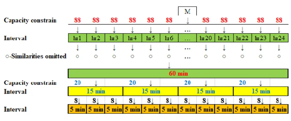
The coordination time interval represents the unit of time (e.g., 5-min, 15-min, 60-min) used as the basis for capacity determination and slot allocation. Usually each time interval contains multiple slots. A movement corresponds to a takeoff or landing activity. A slot refers specifically to the interval occupied by one movement.
Flight implementation difficulties index and difficulty brought by difficulty index expressed as follow:
=⌊ 𝑛 12∙ 32⌋ (1)
=| | ∙ =| | ∙ ⌊ 𝑛 12∙ 32⌋ (2) As mentioned before, cost of one movement in most of traditional slot allocation models is as following:
𝑂 | | ∙ (3)
In expression (3), 𝑂 is the interval displacement when required interval is replaced with scheduled interval .
When priority is considered as the cost of displacing the unit time, cost of one movement can be presented as following:
𝑃 | | ∙ (4)
In our model, we integrate cost of displacement, difficulties and priorities as a whole in order to facilitate calculation and comparison. At the same time, three weight factors ( ) are introduced artificially for the same reason. Performance comparing under different target weights have been done in our previous articles[24], so this paper sets the weight to [1, 0, 0], only changes the capacity settings in constrains to observe the waveform changes. The comprehensive displacement
cost of a movement, displaced from required interval to scheduled interval , could be expressed as following:
𝛿𝑂 𝑃 ∙ + ∙ + ∙ ∙ + ∙ ⌊( ) ⌋ + ∙ (5)
∙ 𝑂+ ∙ + ∙ 𝑃 | |𝛿𝑂 𝑃 (6) We call 𝛿𝑂 𝑃 as the comprehensive displacement cost factor with the consideration of implementation difficulties and priority. It is important to find that 𝛿𝑂 𝑃 is a constant, which makes it possible to solve the following slot allocation model by Linear Integer Programming (LIP).
minimize ∑ ∑
∑ ∑| | 𝛿𝑂 𝑃
(7)
subject to ∑ =1, (8)
∑ ∑ , c C, ,s (9)
{ } , (10)
The objective function (7) minimizes the overall displacement cost of all flights. Constraint (8) stipulates that every movement must be allocated to one interval. Constraint (9) specifies that total movement consumption cannot exceed capacity, for each constraint, day and interval. Constraint (10) ensures that this model can be solved by integer programming method. There is no detailed description of the coefficient matrix in previous papers. Thus, in the next section, we will elaborate proposed approach.
3 LIP for slot displacement models
In order to limit the flow of corridors, it is necessary to determine which corridor should be allocated to each flight. Firstly, the courses of all flights from the airport to the linked airport are calculated. Then, the courses for arrival or departure are sorted descending. If there are m corridors for arrival (or departure), then the arrival (or departure) courses are classified into m categories.
In general, the number of corridors for arrival is equal to the number of corridors for departure.
Each corridor entrance must meet the capacity constraints. All movement is classified according to the number of corridors and assigned evenly to corridor before executing LIP. By designing the variable yie { } i M e E, the relationship matrix of movement and corridors is constructed as shown in table 1. The sum of each column must be 1, that is, each movement i must be assigned to a corridor e. The sum of each row is limited by the capacity of the corridor in every interval. This makes it easy to solve the capacity constraints of the corridor with linear programming, but with the increase of the number of flights and the number of corridors, the dimension of the constraints increases rapidly.
Table 1. relationship matrix of movement i and corridors e
e i 1 2 3 4 … M
1 1 0 0 0 … 0
2 0 0 1 0 … 1
3 0 0 0 0 … 0
… … … …
E-1 0 0 0 1 … 0 𝐸−
E 0 1 0 0 … 0 𝐸
Considering that the flight execution cycle is usually at least once a week, and that most flights operate every day, in order to reduce the computing time with the proposed approach, it is possible to determine the calendar days with the same set of requests, and then represent these as a single calendar day. In order to keep the accumulated rolling volume of flights from exceeding the hourly capacity, we consider three kinds of capacities in brackets (hourly capacity, 15-minutes capacity and 5-minutes capacity) to prevent this from happening. For preventing memory overflow, these three capacities are arranged separately and in the order of hourly capacity, 15-minutes capacity and 5-miute capacity sequentially, that is to say, the other two are not active in the arrangement of the third capacity. Because of the fact that 5-minutes capacity has greatest effect on the uniform distribution of time, the check of 5-minutes capacity is put at the end. When constrains of 5-minutes capacity is check, the dimension of the constraint is so large that sometimes the memory is insufficient to execute. Therefore, we activate constrains of runway capacity and corridors capacity in batches according to the order of priority. The corresponding capacity is updated after each batch of arrangement. This top-down decomposition of these constraints is shown in Figure 3.
There are five ways to feed data for equation (9) in order to split data and reduce memory requirements.
(1) The first is to satisfy capacity constraints from top to bottom, as we do, which is equivalent to allocating applications to each hourly interval according to the hourly capacity constraints. On the basis of the results, as many applications as possible are allocated to 15-minutes intervals in batches according to 15-minutes capacity constraints.
Finally, on the basis of the previous results, according to the 5-minutes capacity constraints, as many applications are allocated to 5-minutes intervals in batches as possible. This feeding process is shown in Figure 1.
Figure 1. Data feeding method 1
(2) The second is to consider three capacity constraints at the same time. Data feeding method of this kind is shown in Figure 2.
Figure 2. Data feeding method 2
(3) The third is to satisfy capacity constraints from top to bottom as the first one, which is equivalent to allocating applications to each hourly point according to the hourly capacity constraints. This stage is the same as the first method. Then, according to the 15-minutes capacity constraints, the application within one hour is allocated to the 15-minutes time points, and finally the application within 15 minutes is allocated to the 5-minutes time points according to the 5-minutes capacity constraints. Data feeding method of this kind is shown in Figure 3.
Figure 3. Data feeding method 3 (4) The fourth is to reverse the first method of feeding.
(5) The fifth is to reverse the third method of feeding.
It is obvious that the first data feeding method is better than the third and fifth methods, because the more applications are fed each time, the greater the possibility of approaching the global optimum. Similarly, the fourth method is better than the fifth one.
T
he first data feeding method is better than the fourth method, because by controlling the application volume in a small interval makes it impossible to overcapacity in a large interval with the first data feeding method. Conversely, small interval may exceed capacity with the fourth data feeding method. The first is better than the second, which we will discuss at the end. So we use the data feeding method 1 in procedures of slot allocation.The following is the procedures of iterative linear integer programming algorithms based on data-splitting method 1.
Column generation procedure
Priority calculation 𝑃 For i=1:7
Load movement in day 1
Set up hourly capacity C60, 15-minutes capacity C15, 5-minutes capacity C5 Calculating the minimum total capacity, Z=Min (24×C60, 96×C15, 288×C5)
Compared with M and Z, if M is larger than Z, the number of discarded requests is equal to M-Z Use simplex method to arrange all remaining applications into each hourly period
Use simplex method to arrange the 15-minutes period on the basis of the hour schedule Use simplex method to arrange the 5-minutes period on the basis of the 15-minutes schedule End
Table 2 is an example of describing the coefficient matrix in detail in the objective function and constrains within hours.
Table 2. Coefficient matrix and detailed expression when slot is based on hour
Execution batch equals P=⌊ /𝑄⌋
∑ ∑
∑ ∑| | 𝛿 𝑃
= + + +⋯+ 4 4+
+ + +⋯+ 4 4+
⋯
+ + +⋯+ 4 4
(a.0)
∑ ∑ , c , , S
𝑨𝟏
+ + +⋯+ ≤ (a.1)
+ + +⋯+ ≤ (a.2)
⋮ ⋮
4+ 4+ 4+⋯+ 4≤ 4 (a.24)
∑ ∑ , c ,corridor 1
, S
𝒀
𝑦 +𝑦 +𝑦 +⋯+𝑦 ≤ (b.1)
𝑦 +𝑦 +𝑦 +⋯+𝑦 ≤ (b.2)
⋮ ⋮
𝑦 4+𝑦 4+𝑦 4+⋯+𝑦 4≤ 4 (b.24)
⋮ ⋯ ⋮ ⋮ ⋮ ⋯ ⋮ ⋮ ⋮
∑ ∑ , c ,corridor 8
, S
𝑦8 +𝑦8 +𝑦8 +⋯+𝑦8 ≤ 8 (b.169)
𝑦8 +𝑦8 +𝑦8 +⋯+𝑦8 ≤ 8 (b.170)
⋮ ⋮
𝑦8 4+𝑦8 4+𝑦8 4+⋯+𝑦8 4≤ 8 4 (b.216)
∑ =1, 𝑄 { } 𝑄
𝑨𝒆𝒒
+ + +⋯+ 4=1
+ + +⋯+ 4=1
⋮
+ + +⋯+ 4=1
(d.1)
(d.2)
⋮
(d.m)
4 Testing results and analysis of the effect of capacity setting on waveform of slot
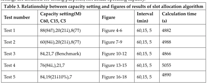
The purpose of the test covers two folds. First is to observe the feasibility and efficiency of the proposed algorithm. Secondly, by changing the hourly capacity, 15-minutes capacity and 5-minutes capacity, the change of flight wave structure can be observed and analyzed. Test parameter setting is show in Table 3. The test data comes from the OAG database. The data is the actual operation data, not the schedule data, and only part of the data for a week, with 1418 movements per day. Capacity settings are assumed for testing purposes, not actual operating capacity.
Table 3. Relationship between capacity setting and figures of results of slot allocation algorithm Test number Capacity setting(M)
C60, C15, C5 Figure Interval
(min)
Calculation time (s)
Test 1 88(84↑),20(21↓),8(7↑) Figure 4-6 60,15, 5 4882 Test 2 60(84↓),20(21↓),8(7↑) Figure 7-9 60,15, 5 4988 Test 3 84,21,7 (Benchmark) Figure 10-12 60,15, 5 4866
Test 4 76(84↓,),21,7 Figure 13-15 60,15, 5 5055
Test 5 84,19(21↓10%),7 Figure 16-18 60,15, 5 4890
Test 6 84,23(21↑10%,),7 Figure 19-21 60,15, 5 4846
Test 7 88(84↑5%),21,7 Figure 22-24 60,15, 5 4850
Test 8 88(84↑5%),23(21↑10%),7 Figure 25-27 60,15, 5 4848 Test 9 88(84↑5%),18(21↓14%),7 Figure 28-30 60,15, 5 4896
4.1 Figures of results of slot allocation algorithm with different virtual capacity setting There are eight tests in total, and each test produces a timetable. The hour distribution, 15-minutes distribution and 5-minutes distribution of the timetable are plotted and shown in the figures resulting from following tests.
4.1.1 Test 1: three kind of capacity set as 88(84↑),20(21↓),8(7↑)
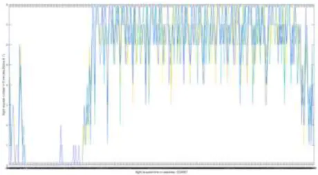
Figure 4. The hourly wave of capacity set as 88,20,8
Figure 5. The 15minutes wave of capacity set as 88,20,8
Figure 6. The 5minutes wave of capacity set as 88,20,8 4.1.2 Test 2: three kind of capacity set as 60(84↓),20(21↓),8(7↑)
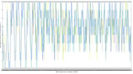
Figure 7. The hourly wave of capacity set as 60,20,8
Figure 8. The 15minutes wave of capacity set as 60,20,8
Figure 9. The 5minutes wave of capacity set as 60,20,8
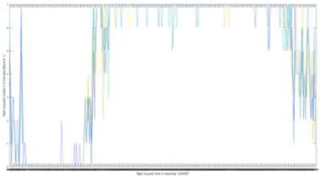
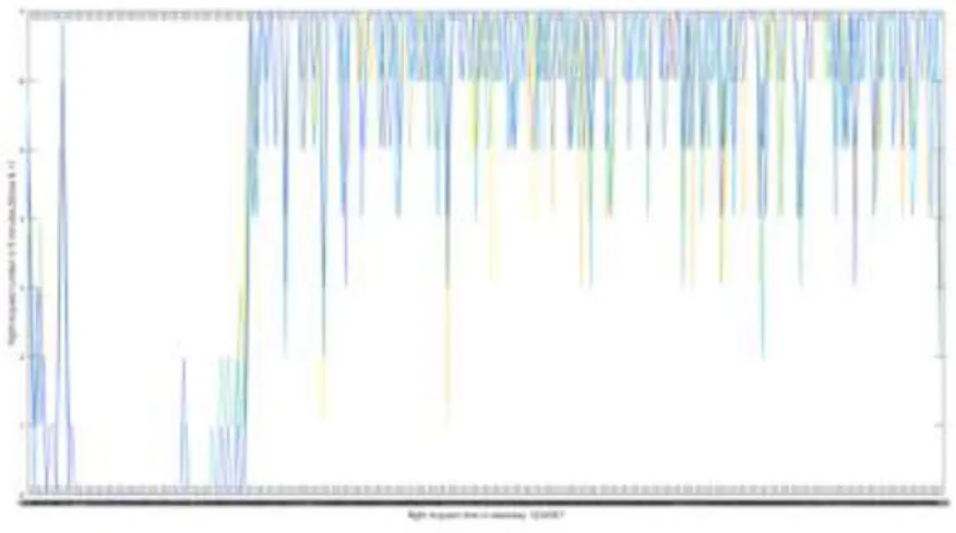
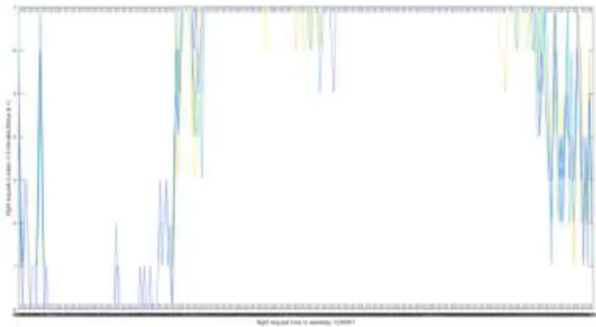
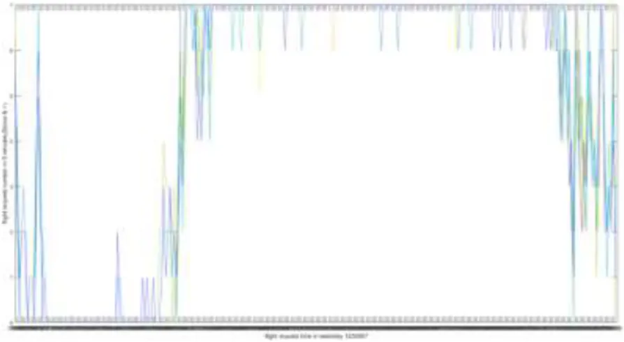
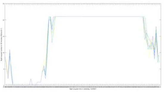
4.1.3 Test 3: three kind of capacity set as 84,21,7 (Benchmark)
Figure 10. The hourly wave of capacity set as 84,21,7
Figure 11. The 15minutes wave of capacity set as 84,21,7
Figure 12. The 5minutes wave of capacity set as 84,21,7 4.1.4 Test 4: three kind of capacity set as 76(84↓10%),21,7
Figure 13. The hourly wave of capacity set as 76(84↓10%),21,7
Figure 14. The 15minutes wave of capacity set as 76(84↓10%),21,7
Figure 15. The 5minutes wave of capacity set as 76(84↓10%),21,7 4.1.5 Test 5: three kind of capacity set as 84,19(21↓10%),7
Figure 16. The hourly wave of capacity set as 84,19(21↓10%),7
Figure 17. The 15minutes wave of capacity set as 84,19(21↓10%),7
Figure 18. The 5minutes wave of capacity set as 84,19(21↓10%),7
4.1.6 Test 6: three kind of capacity set as 84,23(21↑10%,),7
Figure 19. The hourly wave of capacity set as 84,23,7
Figure 20. The 15minutes wave of capacity set as 84,23,7
Figure 21. The 5minutes wave of capacity set as 84,23,7 4.1.7 Test 7: three kind of capacity set as 88(84↑5%),21,7
Figure 22. The hourly wave of capacity set as 88(84↑5%),21,7
Figure 23. The 15minutes wave of capacity set as 88(84↑5%),21,7
Figure 24. The 5minutes wave of capacity set as 88(84↑5%),21,7
4.1.8 Test 8: three kind of capacity set as 88(84↑5%),23(21↑10%),7
Figure 25. The hourly wave of capacity set as 88,23(21↑10%),7
Figure 26. The 15minutes wave of capacity set as 88,23(21↑10%),7
Figure 27. The 5minutes wave of capacity set as 88,23(21↑10%),7
4.1.9 Test 9: three kind of capacity set as 88(84↑5%),18(21↓14%),7
Figure 28. The hourly wave of capacity set as 88(84↑5%),18(21↓14%),7
Figure 29. The 15minutes wave of capacity set as 88(84↑5%),18(21↓14%),7
Figure 30. The 5minutes wave of capacity set as 88(84↑5%),18(21↓14%),7 4.2 Analysis of the effect of capacity setting on waveform of slot
From the results of test 1-8, we found that slot wave has specific characteristics under different capacity setting as following Table 4.
Table 4. Characteristics of slot wave under different capacity setting
Test [C60, C15, C5]
(U, V, W) Relationship Waveform characteristics
Ā𝟏 Ѱ𝟏
ω
Ā𝟐 Ѱ𝟐
ω
Ā𝟑 Ѱ𝟑
ω
1 [88,20,8]
(88,80,96)
V< U<W C15< R< Q
T< S< C5
Lots of shock waves are capped by [U,Q,C5]
Ā =V ѱ≤U-V
Ā =C15 ѱ≤Q-C15
Ā =T ѱ≤C5-T
2 [60,20,8]
(60,80,96)
U<V<W R<C15<Q
S<T<C5
Lots of shock waves are capped by [U,R,S]
Ā = U ѱ≤V-U
Ā= R ѱ≤Q-R
Ā =S ѱ≤C5-S
3 [84,21,7]
(84,84,84)
U=V=W R=C15=Q
S=T=C5
A few sawtooth waves are capped by [U, R, S]. The amplitude of this kind of wave is very small in busy period.
Ā = U=V=W ѱ=0 ω≤ U ω| 𝑝→0
Ā =Q=R=C15 ѱ=0 ω≤ R ω| 𝑝→0
Ā =T=C5 ѱ=0 ω≤ S ω | 𝑝→0
4 [76,21,7]
(76,84,84)
U<V=W R<C5=Q
S<T=C5
Lots of shock waves are capped by [U,R,S]
Ā = U ѱ≤V-U
Ā= R ѱ≤Q-R
Ā =S ѱ≤C5-S
5 [84,19,7]
(84,76,84)
V<U=W C15<R=Q
T<S=C5
Lots of shock waves are capped by [W,Q,C5]
Ā= V ѱ≤W-V
Ā =C15 ѱ≤Q-C15
Ā =T ѱ≤C5-T
6 [84,23,7]
(84,92,84)
U=W<V R=Q<C15
S=C5<T
A few sawtooth waves are capped by [U, R, S]. The amplitude of this kind of wave is very small in busy
Ā = U ѱ=0 ω≤U ω| 𝑝→0
Ā= R ѱ=0 ω≤ R ω| 𝑝→0
Ā =S ѱ=0 ω≤ S ω | 𝑝→0
period.
7 [88,21,7]
(88,84,84)
W=V<U C15=Q<R
T=C5<S
A few sawtooth waves are capped by [W,Q,C5]. The amplitude of this kind of wave is very small in busy period.
Ā=W ѱ=0 ω≤ W ω| 𝑝→0
Ā=Q ѱ=0 ω ≤ Q ω| 𝑝→0
Ā =C5 ѱ=0 ω≤ C5 ω | 𝑝→0
8 [88,23,7]
(88,92,84)
W<U <V Q<R<C15
C5<S<T
Very few sawtooth waves are capped by [W,Q, C5].
The amplitude of this kind of wave almost disappears in busy period.
Ā=W ѱ=0 ω≤ W ω| 𝑝→0
Ā=Q ѱ=0 ω ≤ Q ω| 𝑝→0
Ā =C5 ѱ=0 ω≤ C5 ω | 𝑝→0
9 [88,18,7]
(88,72,84)
V <W<U C15<Q<R
T<C5<S
Lots of shock waves are capped by [W,Q,C5]
Ā= V ѱ≤W-V
Ā =C15 ѱ≤Q-C15
Ā =T ѱ≤C5-T
*Notation: U= C60 (60min);V= C15×4(60 min);W= C5×12(60 min);Q= C5×3(15 min);R= C60÷4(15 min);S= C60÷12(5 min);T= C15÷3(5 min); Ā is Hourly wave oscillation axis; Ā is 15-minutes wave oscillates axis; Ā is 5-minutes wave oscillates axis; Ѱ is upper half amplitude of hourly wave; Ѱ is upper half amplitude of 15-minutes wave; Ѱ is upper half amplitude of 5-minutes wave.
Bp: busy period
From the Table 4 we can see that wave oscillates around Ā =min[U,V,W] , Ā =min[R,C15,Q], Ā=min[S, T, C5] and they are all capped by their second largest number.
Test 1-9 are classified according to the characteristic parameters of the wave and are shown in Table 5. The waveforms of class 1-3 are similar, but the characteristic parameters are slightly different.
So do class 4-5. Class 3, 6, 7, 8 can be categorized into one group (W≤V) and class 2, 4, 1, 5, 9 can be categorized into another group (V≤W) when classification is based on the shape of the wave.
Table 5. Classification of tests according to characteristic parameters of the wave and grouping according to shape of the wave
Class
Ā𝟏
Ѱ𝟏 ω
Ā𝟐
Ѱ𝟐 ω
Ā𝟑
Ѱ𝟑 ω
Waveform characteristics Relationship Test group
1
Ā= U=V=W ѱ=0 ω≤ U ω| 𝑝→0
Ā =Q=R=C15 ѱ=0 ω≤ R ω| 𝑝→0
Ā =T=C5 ѱ=0 ω ≤ S ω | 𝑝→0
A few sawtooth waves are capped by [U, R, S]. The amplitude of this kind of wave is very small in busy period.
U=V=W 3
W≤V 2
Ā= U ѱ=0 ω≤U ω| 𝑝→0
Ā = R ѱ=0 ω≤ R ω| 𝑝→0
Ā =S ѱ=0 ω ≤ S ω | 𝑝→0
A few sawtooth waves are capped by [U, R, S]. The amplitude of this kind of wave is very small in busy period.
U=W<V 6
3
Ā=W ѱ=0 ω≤ W ω| 𝑝→0
Ā =Q ѱ=0 ω≤ Q ω| 𝑝→0
Ā =C5 ѱ=0 ω ≤ C5 ω | 𝑝→0
A few sawtooth waves are capped by [W,Q,C5]. The amplitude of this kind of wave is very small in busy
W=V<U
W<U <V 7,8
period.
4 Ā= U ѱ≤V-U
Ā = R ѱ≤Q-R
Ā =S ѱ≤C5-S
Lots of shock waves are capped by [U,R,S]
U<V<W
U<V=W 2,4
V<W 5 Ā=V
ѱ≤U-V
Ā =C15 ѱ≤Q-C15
Ā =T ѱ≤C5-T
Lots of shock waves are capped by [U,Q,C5] or [W,Q,C5]
V< U<W V<U=W V <W<U
1,5,9
*Notations are same as table 4.
5 Discussion
5.1 Memory consumption analysis
If the hourly capacity, 15-minutes capacity and 5-minutes capacity constraints are met at the same time, the capacity constraints in expression (9) must be based on Table 6. And expression (9) is expanded in the following three expressions (11-13).
Table 6. Coefficient Matrix using in Capacity constrains M S 1 2 … 288 Variable constrains
1 x11 x12 … x1288 1
2 x21 x22 … x2288 1
3 x31 x32 … x3288 1
… … … … …
m xm1 xm2 … xm288 1
The 5-minutes capacity constraints are as following:
∑ 𝑖𝑗
𝑖=
(11)
The 15-minutes capacity constraints are as following:
∑ 𝑖𝑗
𝑖=
+ ∑ 𝑖 𝑗+
𝑖=
+ ∑ 𝑖 𝑗+
𝑖=
(12)
The hourly capacity constraints are as following:
∑ 𝑖𝑗
𝑖=
+ ∑ 𝑖 𝑗+
𝑖=
+ ⋯ + ∑ 𝑖 𝑗+
𝑖=
(13)
Obviously, if three kinds of capacity constrains must be met at the same time, the memory consumption will increase greatly, and the number of applications that can be fed at one time will greatly reduce. This implies that the optimization effect will be reduced, and the minimum value in [C60, C15×4, C5×12] will play a dominant role in these constraints.
On the contrary, the capacity constraints used in our algorithm are much simpler. Three kinds of capacity constraints are shown as following in the sequence hourly, 15 minutes and 5 minutes.
∑ 𝑖𝑗
𝑖=
(14)
∑ 𝑖𝑗
𝑖=
(15)
∑ 𝑖𝑗 𝑖=
(16)
Data feeding method used in our algorithm not only simplifies the coding, but also reduces the dimension of constraints. This implies that the optimization effect will be increased, because of the fact that more applications can be fed to the program at a time.Therefore, by combining the previous analysis in section 3, it can be concluded that the data feeding method 1 is better than the second one, and it is the best of the five data feeding methods proposed in section 3.
Since there is no detailed description of data feeding method in previous articles, it is difficult to compare optimization effect with previous methods. But, based on the analysis of possible data splitting methods, we still could figure out which data feeding method is good or bad from the feedable data quantity. In the future research, we need to use test data to prove which data feeding method proposed in section 3 has the best optimization effect.
Our LIP algorithm was solved by MATLAB 2018. All tests were run on a desktop with 16 GB RAM and AMD RYZEN 5 1600 6-Core 3.2 GHz. According to table 3, using our LIP algorithm based on the first data feeding method, the average computing time was 1.36 hours per time with 9926 applications in 7 days, and was 12 minutes per time with 1418 applications per day. The calculation time includes the time to read and write excel files. The most time-consuming function in profile summary report for our LIP algorithm is the ‘matrixconfig’ function for constructing constraints matrix, as shown in Figure 31.
Figure 31. Profile summary report for our LIP algorithm
5.2 Effect of virtual capacity setting on slot waveform based on our the data feeding method
By observing the waveforms of these different capacity settings, we observed that according to our slot allocation algorithm based on the data feeding method 1, different settings of the three kinds of capacities have dominant effect on the waveform. Through nine tests and analyses in section 4, some interesting findings are as follows.
A. The most important finding is that under the data feeding mode we choose, there is no shock wave in busy period when W ≤V, but when W ˃V, there will be shock wave in busy period.
B. Three kinds of shock waves exist or do not exist at the same time with different capacity setting.
C. Three kinds of shock waves oscillates around Ā=min[U,V,W], Ā=min[R,C15,Q], Ā=min[S, T, C5] and they are all capped by their second largest number.
D. When there is a shock wave, the amplitude of hourly wave is proportional to |U V|.
Hourly wave oscillates around Ā =min[U,V,W]. The 15-minutes wave oscillates around Ā =min[R,C15,Q]. The 5-minutes wave oscillates around min[S, T, C5].
6 Conclusion
The data feeding method 1 is the best in five data feeding methods proposed in section 3.
Computing time of our LIP algorithm is acceptable.The amplitude of the wave could be controlled to wanted range by the capacity setting. In this way, the rolling capacity constrains could be avoided and the computing time and complexity could be greatly reduced. It solves the problem that LIP is difficult to be used in large-scale slot allocation because of prohibited memory consuming.
Our study suggests that the proposed methods could be used to control and design the amplitude of the slot wave. This means that virtual capacity settings could be used to control demand within declared capacity. Our research also provides clues for further research on the construction of the flight waves to improve the hit rate[25]. It is hopeful to further improve the reliability of the flight waves for airlines operating at specific airports in order to establish direct or indirect connectivity, and increase hit rate by choosing preferred virtual capacity settings. In addition, the precise quantitative relationship between the period, the phase of waves and capacity setting needs to be further studied.
Acknowledgements
This work is supported by the National Natural Science Foundation of China (grant number 71571182), the National Natural Science Youth Foundation of China (grant number 61603396), the National Natural Science Foundation of China and the Civil Aviation Grant (grant number U1633124) and the research projects of the social science, humanity on Young Fund of the ministry of Education of China (grant number 14YJC630185) and the Fundamental Research Funds for the Central Universities (grant number ZXH2011C009).
Referance
[1] Zografos KG, Madasz MA, Salourasx Y. A decision support system for total airport operations management and planning. J Adv Transport. 2013;47(2):170-89.
[2] Barnhart C, Fearing D, Odoni A, Vaze V. Demand and capacity management in air transportation.
EURO Journal on Transportation and Logistics. 2012;1(1):135-55.
[3] Jacquillat A, Odoni AR. An Integrated Scheduling and Operations Approach to Airport Congestion Mitigation. Operations Research. 2015;63(6):1390-410.
[4] Zografos KG, Salouras Y, Madas MA. Dealing with the efficient allocation of scarce resources at congested airports. Transportation Research Part C-Emerging Technologies. 2012;21(1):244-56.
[5] Zografos KG, Madas MA, Androutsopoulos KN. Increasing airport capacity utilisation through optimum slot scheduling: review of current developments and identification of future needs. J Scheduling. 2017;20(1):3-24.
[6] Basso LJ, Zhang AM. Pricing vs. slot policies when airport profits matter. Transport Res B-Meth.
2010;44(3):381-91.
[7] Verhoef ET. Congestion pricing, slot sales and slot trading in aviation. Transport Res B-Meth.
2010;44(3):320-9.
[8] Zhang AM, Zhang YM. Airport capacity and congestion pricing with both aeronautical and commercial operations. Transport Res B-Meth. 2010;44(3):404-13.
[9] Czerny AI, Zhang AM. Airport congestion pricing and passenger types. Transport Res B-Meth.
2011;45(3):595-604.
[10] Le L, Donohue G, Hoffman K, Chen CH. Optimum airport capacity utilization under congestion management: A case study of New York LaGuardia airport. Transport Plan Techn. 2008;31(1):93-112.
[11] Vaze V, Barnhart C. Modeling Airline Frequency Competition for Airport Congestion Mitigation.
Transportation Science. 2012;46(4):512-35.
[12] Jacquillat A, Odoni AR. Congestion Mitigation at John F. Kennedy International Airport in New York City: Potential of Schedule Coordination. Transport Res Rec. 2013(2400):28-36.
[13] Pyrgiotis N, Odoni A. On the Impact of Scheduling Limits: A Case Study at Newark Liberty International Airport. Transportation Science. 2016;50(1):150-65.
[14] Ribeiro NA, Jacquillat A, Antunes AP, Odoni AR, Pita JP. An optimization approach for airport slot allocation under IATA guidelines. Transport Res B-Meth. 2018;112:132-56.
[15] Zografos KG, Androutsopoulos KN, Madas MA. Minding the gap: Optimizing airport schedule displacement and acceptability. Transportation Research Part A: Policy and Practice. 2018;114:203-21.
[16] Jacquillat A, Odoni AR. Endogenous control of service rates in stochastic and dynamic queuing models of airport congestion. Transportation Research Part E-Logistics and Transportation Review.
2015;73:133-51.
[17] Jacquillat A, Odoni AR. A roadmap toward airport demand and capacity management.
Transportation Research Part a-Policy and Practice. 2018;114:168-85.
[18] Benlic U. Heuristic search for allocation of slots at network level. Transportation Research Part C-Emerging Technologies. 2018;86:488-509.
[19] Li X, Chen X, Li D, Wei D. Classification and characteristics of flights taking off and landing waveforms. FLIGHT DYNAMICS. 2016;34(02):90-4.
[20] Sun CL, Su X. Analysis & Optimization of Beijing Capital Airport's flight waves. China Civil Aviation. 2013(10):30-1.
[21] Hu M, Yi T, Ren Y. Optimization of airport slot based on improved Hungarian algorithm.
Application Research of Computers. 2019(08):1-7.
[22] Huang J, Wang J. A comparison of indirect connectivity in Chinese airport hubs: 2010 vs. 2015.
Journal of Air Transport Management. 2017;65:29-39.
[23] Jacquillat A, Vaze V. Interairline Equity in Airport Scheduling Interventions. Transportation Science. 2018;52(4):941-64.
[24] Ye ZL, Y.; Bai, J.; Zheng, X. Performance Comparing and Analysis for Slot Allocation Model.
Preprints 20192019.
[25] Goedeking P. Networks in aviation: Strategies and structures. Expert Opinion on Biological Therapy. 2010;8(2):213.