Multialternative decision by sampling : a model of decision making constrained by process data

warwick.ac.uk/lib-publications

Original citation:

Noguchi, Takao and Stewart, Neil (2018) Multialternative decision by sampling : a model of

decision making constrained by process data. Psychological Review, 125 (4). pp. 512-544.

doi:10.1037/rev0000102

Permanent WRAP URL:

http://wrap.warwick.ac.uk/97406

Copyright and reuse:

The Warwick Research Archive Portal (WRAP) makes this work of researchers of the

University of Warwick available open access under the following conditions.

This article is made available under the Creative Commons Attribution 3.0 (CC BY 3.0) license

and may be reused according to the conditions of the license. For more details see:

http://creativecommons.org/licenses/by/3.0/

A note on versions:

The version presented in WRAP is the published version, or, version of record, and may be

cited as it appears here.

Multialternative Decision by Sampling: A Model of Decision Making

Constrained by Process Data

Takao Noguchi

Neil Stewart

Sequential sampling of evidence, or evidence accumulation, has been implemented in a variety of models to explain a range of multialternative choice phenomena. But the existing models do not agree on what, exactly, the evidence is that is accumulated. They also do not agree on how this evidence is accumulated. In this article, we use findings from process-tracing studies to constrain the evidence accumulation process. With these constraints, we extend the decision by sampling model and propose the multialternative decision by sampling (MDbS) model. In MDbS, the evidence accumulated is outcomes of pairwise ordinal comparisons between attribute values. MDbS provides a quantitative account of the attraction, compromise, and similarity effects equal to that of other models, and captures a wider range of empirical phenomena than other models.

Keywords:attraction effect, compromise effect, evidence accumulation, sequential sampling, similarity effect

One overarching idea in decision research is that people accumu-late evidence for alternatives over time, with a decision reached when the evidence reaches a decision criterion. This sequential accumula-tion of evidence has proven effective in explaining neural activity during decision (see, e.g.,Gold & Shadlen, 2007, for review) and in capturing the time course of perceptual judgments (see, e.g.,Ratcliff & Smith, 2004;Teodorescu & Usher, 2013, for reviews). Evidence accumulation provides a general framework for decisions, where values need to be integrated over time or across attributes. Within the multialternative decision making, many implementations of evidence accumulation have been proposed, as listed inTable 1.

One primary difference between the models concerns what, exactly, the evidence is that is accumulated on each step. In some models, transformed attribute values are accumulated. In other models, differences in (raw or transformed) attribute values are

accumulated. Other major differences concern the stochastic fluc-tuation of attention and the choice of decision criterion, as sum-marized inTable 1.

The contribution of this paper is to present a new model, which we call multialternative decision by sampling (MDbS). This model is an extension of decision by sampling (DbS;Stewart, Chater, & Brown, 2006). The MDbS model differs from the other sequential sampling models of multialternative choice primarily in that the evidence accumulated is pairwise ordinary comparisons on single attribute dimensions. For example, consider a decision between cars: a Ford, a BMW, and a Nissan. The Ford may have a lower price than the BMW, resulting in one unit of evidence accumulated for the Ford. Then, in the next step, the Ford beats the Nissan on fuel efficiency, resulting in one unit of evidence accumulated for the Ford. These steps continue until one car is sufficiently far ahead in evidence units, whereupon a choice is made.

We have used findings from process tracing studies, in partic-ular those on eye-movements, to provide some constraints on how evidence is accumulated. The MDbS model is guided by three constraints in particular. First, the existing literature shows that, in multialternative decision, people’s attention fluctuates between pairs of alternatives on single attributes at one time (Russo & Leclerc, 1994;Russo & Rosen, 1975). So, in the MDbS model, the evidence accumulated is the outcome of a series of evaluations of pairs of alternatives on single dimensions. The link between the attention fluctuation and decision is reported in process-tracing studies (Noguchi & Stewart, 2014;Stewart, Gächter, Noguchi, & Mullett, 2016). The second constraint is that more similar alterna-tives receive more attention (Noguchi & Stewart, 2014). So, in the MDbS model, more similar alternatives are more likely to be selected for comparison. Third, the distribution of time taken to make a decision (response time) is generally positively skewed and, toward the end of a decision, people attend more to the alternative which they are going to choose (the gaze cascade effect; Shimojo, Simion, Shimojo, & Scheier, 2003; Simion & Shimojo, 2007).Mullett and Stewart (2016)show, in a series of simulations, that positively skewed response times and the gaze

Takao Noguchi, Department of Experimental Psychology, University College London; Neil Stewart, Warwick Business School, University of Warwick.

This research was supported by grants from the Economic and Social Research Council ES/K002201/1, ES/K004948/1, ES/N018192/1, and the Leverhulme Trust RP2012-V-022, awarded to Neil Stewart. These funding sources provided financial support but were not involved in any other aspects of the research. We thank Anthony A. J. Marley, Jerome Buse-meyer, and reviewer Michael P. R. Doughery for their comments.

This article has been published under the terms of the Creative Com-mons Attribution License (http://creativecommons.org/licenses/by/3.0/), which permits unrestricted use, distribution, and reproduction in any me-dium, provided the original author and source are credited. Copyright for this article is retained by the author(s). Author(s) grant(s) the American Psychological Association the exclusive right to publish the article and identify itself as the original publisher.

Correspondence concerning this article should be addressed to Takao Noguchi, who is now at School of Electronic Engineering and Computer Science, Queen Mary University of London, London E1 4FZ, United Kingdom. E-mail:[email protected]

© 2018 The Author(s) 2018, Vol. 125, No. 4, 512–544

0033-295X/18/$12.00 http://dx.doi.org/10.1037/rev0000102

cascade effect are consistent only with a decision criteria based on a relative difference in the evidence for each alternative, rather than the absolute evidence for an alternative. So, in the MDbS model, we use a relative decision criteria.

Having used process data to set what would otherwise be arbitrary assumptions about the evidence accumulation in MDbS, we then seek to explain a different set of phenomena: decisions in multialternative choice. Initially we focus upon the so-called big three context effects: the attraction, compromise, and similarity effects. The effects have driven the development of models of multialternative decision because of their theoret-ical importance and because of the challenge in producing a simultaneous account of all three. We will show that the MDbS’s quantitative account of the big three context effects is as good as two key competing models which also have closed-form solutions for decision probability: multialternative deci-sion field theory (MDFT;Roe, Busemeyer, & Townsend, 2001) and the multiattribute linear ballistic accumulator model (MLBA; Trueblood, Brown, & Heathcote, 2014). We then broaden our consideration of phenomena using a systematic literature survey, and consider the ability of the MDbS model, and other models, to capture the breadth of phenomena. The MDbS model captures almost all of these phenomena without any further assumptions. To begin, we describe the MDbS model.

Multialternative Decision by Sampling

Overview

In the MDbS model, evidence is accumulated from a series of ordinal comparisons of pairs of attribute values. The attribute values are drawn from the current choice and from long-term memories of attribute values encountered previously. For example, in evaluating the price of Car A people may compare the price against prices sampled from other alternatives in a choice set: the price of Car B also on offer. People may also compare the price of

Car A against prices sampled from long-term memory: prices of other cars they have seen before. No matter the source of the comparison attribute, if the price of Car A is preferable in the pairwise comparison, one unit of evidence is accumulated toward deciding on Car A. This pairwise comparison is considered ordi-nal, in the sense that evidence is increased one single unit amount regardless of how large the difference is. These ordinal compari-sons of pairs of attribute values are sequentially sampled, and drive the evidence accumulation process until the evidence for one alternative is sufficiently far ahead of the evidence for the other alternatives. Below, we expand on this overview.

Working Memory

In the original DbS model, and in MDbS, working memory con-tains the attribute values from the choice set and may also contain attribute values retrieved from long-term memory. All of the attribute values, regardless of their source, are processed in exactly the same way.G. D. A. Brown and Matthews (2011)andTripp and Brown (2015)have integrated a computational model of memory with deci-sion by sampling, but this complexity is not needed to explain the multialternative decisions in this article. Here, working memory is simply the pool of attribute values the decision maker has in the front of their mind. We will see how context effects caused by the addition or removal of alternatives from the current choice set and context effects caused by exposure to attribute values before the current choice are explained by the same mechanism in MDbS.

Similarity Dependent Comparison Probability

In the earlier formulation of the DbS model, all attribute value comparisons are equally likely. But process tracing studies suggest that context influences people’s attention. For example, eye-movement studies find that people attend more frequently to alternatives which share attribute values with other alternatives or have similar attribute values (Noguchi & Stewart, 2014;Russo & Rosen, 1975).Figure 1shows the number of eye-fixation transi-Table 1

Evidence Accumulation Models in Decision Making

Model Evidence accumulated Stochastic attention Decision criterion

AAM Transformed values on one attended attribute One attribute is stochastically selected for each step of evidence

accumulation

Absolute threshold

LCA Differences in transformed attribute values, aggregated over attributes Not assumed External stopping time MADDM Pre-choice attractiveness ratings, weighted by visual attention One alternative is selected for each step

of evidence accumulation

Relative threshold

MDFT Differences in attribute values between the alternative and the average of the other alternatives, on one attribute

One attribute is stochastically selected for each step of evidence

accumulation

Relative threshold

MLBA Differences in transformed attribute values, aggregated over attributes Not assumed Absolute threshold

RN Transformed attribute values, aggregated over attributes Not assumed Not specified

MDbS Ordinal comparisons between a pair of alternatives on single dimensions

A pair and an attribute are stochastically selected for each step of evidence accumulation

Relative threshold

tions between the three alternatives from an experiment by Nogu-chi and Stewart (2014) which presented attraction, compromise, and similarity choices, using different cover stories for each choice. The most frequent transitions are between the most similar alternatives. We describe the attraction, similarity, and compro-mise effects below in detail, but for now note that in the attraction choice set {A, B, D}, transitions are most frequent between pair A and D, prior to a decision. In the compromise choice set {A, B, C}, transitions are most frequent between pair A and B and pair A and C. In the similarity choice set {A, B, S}, transitions are most frequent between pair B and S.

Therefore, in MDbS, the probability of evaluating the value of AlternativeAon Dimensioniis proportional to the similarity to the other attribute values in working memory:

p(evaluateAi)⬀

兺

X_i⫽A_i X_i僆⺣i

exp

共

兲

whereAiis the attribute value for AlternativeAon Dimensioni,⺣i is the set of attribute values from Dimensioniin working memory, andDis a distance function discussed below.

In MDbS, the probability of evaluating A against B can be different to the probability of evaluating B against A. When averaging over the direction of comparison, MDbS produces the qualitative pattern of comparison frequencies illustrated in Fig-ure 1. The gray dots represent predicted frequencies. In a similarity choice, for example, Equation 1 will assign higher evaluation probabilities to Alternatives B and S than to Alter-native A, because B and S both have a high summed similarity to the other alternatives whereas Alternative A does not. Thus, the comparisons which are more frequently made are B against A, B against S, S against A, and S against B. Comparisons of A against B or A against S are less frequent. Because comparisons of B against S and of S against B are both frequent, comparisons

betweenB and S are most frequent, as we see inFigure 1.

Pairwise Ordinal Comparison

In the MDbS model, the rate at which evidence is accumulated for an alternative is determined by two factors: the probability that the alternative is compared on a particular attribute dimension (as described in the previous section), and the probability that the alternative wins the comparison. Formally, the accumulation rate for Alternative A is given by:

p(Evidence is accumulated towardA)

⫽

兺

i僆⺔p(evaluateAi)p(Aiwins a comparison)

⫽

兺

i僆⺔

p(evaluateAi)

⫻

冉

兺

X_i⫽A_i Xi僆⺣i

p(Aiis compared against Xi)p(Aiis favored over Xi)

冊

(2)

where⺔is the set of attribute dimensions along which alternatives are described (e.g., price, comfort and fuel efficiency), andAiis the

attribute value of AlternativeAon Dimensioni, and⺣iis the set of attribute values on Dimensioniin working memory.

The pairwise comparison process is supported by process-tracing studies (e.g., Noguchi & Stewart, 2014; Payne, 1976; Russo & Dosher, 1983;Russo & Leclerc, 1994). These studies show that people move their eyes back and forth between a pair of alternatives on one single attribute value before moving on to the next comparison.

Our assumptions about the ordinality of comparisons—that the evidence accumulation is insensitive to the magnitude of differ-ence between compared values—were grounded in findings from the field of psychophysics, as was the case for the original decision by sampling model (seeStewart et al., 2006). For example, pre-vious research demonstrates that people are rather good at discrim-inating stimuli (e.g., vertical lines of different lengths, or auditory tones of different loudness) from one another, but rather poor at Figure 1. The frequencies of eye-fixation transitions between alternatives for the attraction, compromise, and

identifying or estimating the magnitude of the same stimuli (e.g., estimating line length or tone loudness;Laming, 1984;Shiffrin & Nosofsky, 1994;Stewart, Brown, & Chater, 2005), which suggests that ordinal comparisons are relatively easy. In the context of decision making, these studies indicate that people are rather good at judging whether they prefer one attribute value over another, but rather poor at stating exactly how much more they appreciate that attribute value. For example, people are able to clearly state that they prefer the comfort of driving a Mercedes to the comfort of driving a Toyota, but people may not be able to state how much more (e.g., 1.7 times) they prefer the comfort of the Mercedes to the comfort of the Toyota.

Differences as Fractions

People often behave as if differences are perceived as fractions, as embodied in Weber’s Law. Weber’s Law says that the incre-ment which can be added to a stimulus and just noticed is a constant fraction of the stimulus magnitude. In the context of judgment and decision making, Tversky and Kahneman (1981) report that people are willing to make an extra trip to save $5 on a $15 purchase but unwilling to make the same trip to save $5 on a $125 purchase. This finding suggests that the discount is judged as a fraction and not an absolute value. Although the saving is $5 in both cases, the $5 discount is 33% reduction from the price of $15 but is only 4% reduction from the price of $125. The 4% reduction may not be meaningful enough to influence a decision. Consistent with this finding, changing prices by a small fraction often has only a very small impact on sales (Kalwani & Yim, 1992; Kalyanaram & Little, 1994). Also, studies on employees’ judg-ments of salary increases find that the increment expressed in a fraction is a better predictor of employees’ judgments of mean-ingfulness of the increment (Futrell & Varadarajan, 1985; Hene-man & Ellis, 1982) and also employees’ subsequent spending and saving decisions (Rambo & Pinto, 1989).

Thus, in MDbS, the distance betweenAiandXiis defined as a

fraction:

D(A_i,X_i)⫽

|

|

|

. (3)

Although this form will behave pathologically when Xi

ap-proaches zero, it is sufficient for our purposes. This distance function is used above inEquation 1for the probability that an attribute value is selected for comparison. It is also used in Equa-tion 4below for for the probability that an attribute value wins a comparison.

Probability of Winning a Comparison

The probability that the selected attribute value wins a compar-ison (i.e., is favored over another value) is given by

p(Aiis favored overXi)⫽

再

F

_共

共

兲兲

(4)

whereFis a logistic sigmoid function with␤₀⫽0.1 and␤₁⫽50 in the simulations below. These parameter values mean that an advantage of 10% is favored with .50 probability, and that an

advantage of 20% is favored with⬎.99 probability. Our choice of

␤0 ⫽ 0.1 is based on the previous theoretical preposition that people are more sensitive to a difference greater than 10% (Brand-stätter, Gigerenzer, & Hertwig, 2006). In using the logistic func-tion, we are replacing the hard comparison between attribute values in the original DbS model with a softer comparison.

To illustrate the softer comparison, suppose we have two iden-tical attribute values and gradually increase one of them. As the difference between the two values grows, it becomes more likely for the larger value to be favored with the soft comparison. This gradual increase in the probability of favoring the value is not possible with the hard comparison, where a small difference is completely ignored and the larger value suddenly becomes favored when the difference grows sufficiently large. We note, however, thatEquation 4can emulate the hard comparison with extremely large␤1.

Thus far we have defined all of the terms inEquation 2. That is, we have defined what, exactly, the evidence is that is accumulated in MDbS. More detailed walk-throughs of the numerical compu-tation are provided in Appendixes BandC. What remains is to define the stopping rule.

A Relative Stopping Rule, and a Closed-Form Solution

for Decision Probabilities

are more likely to look at the thing they prefer.) In summary, only a relative stopping rule is consistent with the process tracing evidence, and so, in MDbS, we assume a relative stopping rule (see also,Nosofsky & Palmeri, 1997).

For a decision between more than two alternatives, the criterion is likely to be either (a) a difference between the maximum and next-best evidence or (b) a difference between a maximum and a mean-average evidence (for discussion, seeTeodorescu & Usher, 2013). Further experimental work is required to discriminate be-tween these possibilities. Here, for computational feasibility, we assume that a decision is made when a difference between a maximum and a mean-average evidence reaches a threshold␪ ⫽ 0.1. This threshold value means that, on average, 2.5 comparisons are made prior to a decision in attraction, compromise, similarity choices. By conceptualizing the evidence accumulation as a ran-dom walk over accumulator states, we have been able to follow Diederich and Busemeyer (2003) and develop a closed form so-lution for the decision probabilities.Appendix Agives the deriva-tion.

Testing DbS Mechanisms

In this section, we discuss earlier studies which tested the DbS mechanisms. This work focused upon the predictions the DbS model makes when the attribute values in working memory are manipulated.

Incidental Value Effect

In the DbS and MDbS models, the attribute values that happen to be in working memory determine how much a given attribute value contributes to accumulation rates. Suppose that a decision maker happens to have £1, £2, and £7 in working memory. A target value of £5 will win in each pairwise comparison against £1 and £2, but will lose the comparison against £7 (assuming these differences are sufficiently large). Thus the target £5 will win in two out of three comparisons. Then the probability that the £5 alternative wins a comparison is 2/3⫽.67.

More generally, the probability that an attribute value wins a comparison is closely related to its relative rank within values in working memory. A relative rank is the proportion of attribute values to which a target value compares favorably. In the above example, the relative rank of £5 is .67. When a relative rank is high, an attribute value is more likely— by definition—to win a comparison, leading to a higher accumulation rate and ultimately contributing to a higher decision probability for the alternative.

This predicted relation between a relative rank and decision was tested byUngemach, Stewart, and Reimers (2011), who offered a decision between two probabilistic pay-offs to consumers as they left a supermarket. One alternative offered a .55 probability of £0.50 and otherwise nothing; and the other offered a .15 proba-bility of £1.50 and otherwise nothing.Ungemach et al. (2011)used the supermarket receipt as a proxy for the values that the customer had recently experienced and would likely be in his or her working memory. Ungemach et al.’s (2011) results show that the more values on the receipt that fell between the £0.50 and £1.50 prizes, the more likely that the lottery for £1.50 was chosen. According to DbS, this is because when more prices fall between the £0.50 and £1.50 prizes, the relative rank of these prizes differs more. Of

course, the supermarket prices experienced should not have af-fected the lottery decision, but, according to the DbS and MDbS models, because these values remained in working memory at the time of the lottery decision, they affected the relative ranks of £0.50 and £1.50, and thus affected the lottery decision.

Attribute Distribution Effect

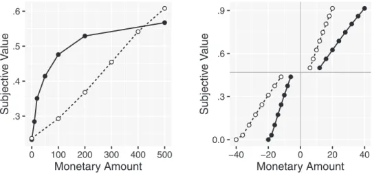
When people are faced with a series of questions, the attribute values from earlier questions can remain in working memory and affect subsequent decisions. Thus different distributions of attri-bute values in earlier questions should have a systematic effect on subsequent decisions. We illustrate this with an example from Stewart, Reimers, and Harris (2015).

Stewart et al. (2015)compared two distributions. In the first, monetary rewards in working memory were positively skewed, with values £0, £10, £20, £50, £100, £200, and £500. In the second, the values were uniformly distributed, with values £0, £100, £200, £300, £400, and £500. Consider one of the attribute values common to both distributions, say £200. In the positively skewed distribution, it has a relative rank of 5/7⫽.71 because it compares favorably to five of the seven attribute values (£0, £10, £20, £50, and £100). In the uniform distribution, it has a relative rank of 2/6⫽.33 because it compares favorably with only two out of the six attribute values (£0 and £100).

Figure 2plots the subjective value functions for money for these positively skewed and uniform distribution conditions. These sub-jective values are computed as the average accumulation rate for the target attribute value (Equation 2). The general principle is that the probability that a target attribute value wins a comparison increases most quickly, and thus a subjective value increases most quickly, in the most dense parts of the attribute value distribution. (Note that the slight deviation from linear for the uniform distri-bution condition and there is also slight variation in the positive skew condition which is harder to see. This is caused by the effects of similarity on the rate at which targets are selected for compar-ison, as is the crossing of the lines near £400 –£500.)

probabilities in the world to inverse-S-shaped weighting functions and the distribution of delays in the world to hyperbolic-like discounting functions. Changes in the distributions of attribute value can also explain key phenomena in risky decision (e.g., the common ratio effect,Stewart & Simpson, 2008;Stewart, 2009).

Loss Aversion

According to the DbS and MDbS models, the distribution of values in working memory offers an explanation of loss aversion. People often behave as if losses loom larger than gains (see Camerer, 2005;Fox & Poldrack, 2014, for reviews). For example, when offered a decision to play gambles with equal chance to win or lose an amount people typically reject such an offer (also see Gal, 2006). Famously, loss aversion was incorporated into the subjective value function in prospect theory (Kahneman & Tver-sky, 1979), which shows a steeper curve in the loss domain than in the gain domain.

In the DbS and MDbS models, loss aversion is explained through an asymmetry in the ranges of the distributions of gains and losses typically used in measuring loss aversion. For example, suppose gains are drawn from a uniform distribution between £0 and £40, but losses are drawn from a uniform distribution between £0 and £20 (e.g., afterTom, Fox, Trepel, & Poldrack, 2007). An increase from £0 to £10 covers one half of the values in the £0 –£20 distribution of losses but only one quarter of the values in the £0 –£40 distribution of gains. Thus the same amount should perceived as larger in losses than gains: people should be more sensitive to losses. When the distributions are reversed so that losses are drawn from a uniform distribution between £0 and £40 and gains are drawn from a uniform distribution between £0 and £20, this sensitivity should also be reversed.

The right panel ofFigure 2shows the predicted subjective value function from the MDbS model, which shows exactly this pattern. These predictions were tested byWalasek and Stewart (2015), who showed the usual loss aversion when the range of losses was

narrower than the range of gains. When gains and losses were symmetrically distributed weak or zero loss aversion was ob-served, and when the distributions were reversed the opposite of loss aversion was observed.

The three phenomena we have reviewed above were designed to test predictions from the DbS model and were run by Stewart and colleagues. Below, we review the empirical findings which were not designed to test the DbS model, and discuss how the MDbS model explains the findings.

The Big Three Context Effects: Attraction,

Compromise, and Similarity

The attraction, compromise, and similarity effects are central to the psychology of multialternative decision because of their theo-retical importance—their very existence rules out the most obvious accounts of how people make decisions. For example, an obvious class of model, foundational in normative economic models of multialternative decision, is the class of simple scalable models. A model has the property of simple scalability if the value of each alternative can be represented by a single scalar (a single real number), with the probability of choosing an alternative increasing in its value and decreasing in the value of other alternatives (see Roe et al., 2001, for a review).

A classic simple scalable model is Luce’s choice rule, where the decision probability for Alternative A is given by p共A

ⱍ

兵A,B,C其兲⫽ VA

VA⫹VB⫹VCwhere theVXs are the values for each of the

X⫽{A,B,C} alternatives. The scalable models have the property that adding an alternative to a choice set cannot reverse the ordering of the decision probabilities for existing alternatives. For example, ifp(A

_|

_|

_|

p(B

_|

ⱍ

VA⫹VB⬎

VB

VA⫹VB⫽p共B

ⱍ

VB, which means p共A

ⱍ

VA⫹VB⫹VC ⬎

VB

VA⫹VB⫹VC ⫽ p

共B

ⱍ

ⱍ

p共B

ⱍ

These scalable models also imply that adding an alternative to a choice set cannot increase the decision probability for any existing alternative: VA

VA⫹VB⫹VCcannot be greater than

VA

VA⫹VBfor any positive

values ofVA,VB, andVC. This property is called regularity. The

properties of independence from irrelevant alternatives and regu-larity are not compatible with the big three context effects: as we discuss below, the big three context effects demonstrate that peo-ple can reverse their relative preference for two alternatives and can become more likely to choose an existing alternative after a new alternative is introduced. Thus the existence of the big three context effects rules out the Luce choice model and all other simple scalable models, such as the Thurstonian model (Thurstone, 1927) and multinomial logistic regression.

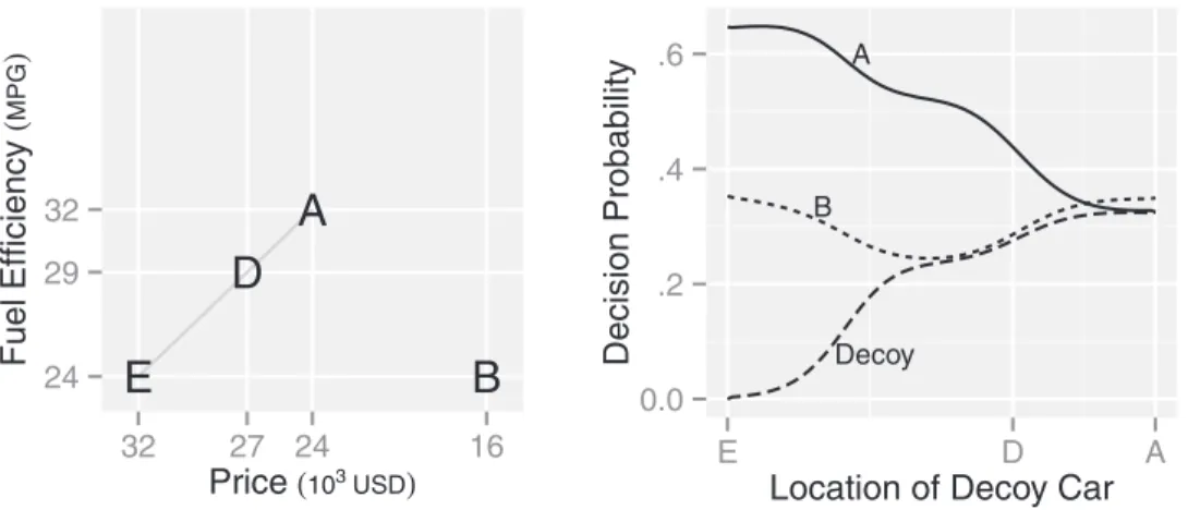
In discussing the big three context effects below, we use an example decision between cars illustrated in the left panel in Figure 3. Available cars are described in terms of the two attri-butes, price (in U.S. dollars) and fuel efficiency (in miles per gallon). Here, Car A is better than Car B on the fuel efficiency but Car B is better than Car A on the price (seeFigure 3). Attribute values were selected from the U.S. car market in May, 2015, such that the MDbS model predicts indifference between Cars A and B when only Cars A and B are in a choice set.

In simulating the big three with the MDbS model, we use a fixed, single set of parameter values throughout this article. We set the similarity parameter ␣ ⫽ 3.0, the soft ordinal comparison parameters for the logistic␤0⫽0.1 and␤1⫽50, and the decision threshold␪ ⫽0.1, as described above. For brevity of explanation, we assume that people are unfamiliar with the choice domain and

cannot sample values from long-term memory beyond those in the immediate choice set. The significance of this assumption is ad-dressed when we discuss how familiarity with choice domain affects the strengths of the context effects.

The Attraction Effect

To illustrate the attraction effect, suppose a choice set contains Cars A, B, and D. Car D is inferior to Car A in both attributes (see the left panel inFigure 3). Thus Car D should be discarded from consideration but, after adding Car D to the choice set, Car A becomes more likely to be chosen than Car B (Huber, Payne, & Puto, 1982). Adding Car D often increases the choice share for Car A, which is a violation of regularity.

While noting that several explanations are possible,Huber et al. (1982)primarily discussed the attraction effect in terms of shifts in weights: addition of Car D would lead people to weight fuel efficiency more heavily as this is where Car D (and also Car A) is advantageous (Huber et al., 1982; see also Bhatia, 2013). This weight-shift account has received mixed support from subsequent studies (e.g.,Wedell, 1991).

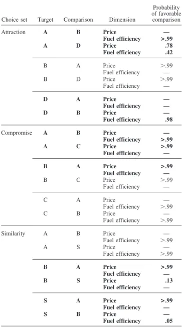
In the MDbS model, however, the attraction effect is explained with changes in the probability of winning comparisons when Car D is added. Table 2 has 12 rows that correspond to all of the possible pairwise comparisons in the attraction effect choice set (three cars can be target⫻two cars can be comparisons for each target⫻two dimensions). The addition of Car D in a choice set increases the probability that Car A wins attribute value compar-isons, because Car A compares favorably with Car D on both price and fuel efficiency, whereas Car B only compares favorably on price. Also, as Cars A and D are similar, they are selected as

targets for comparison more often, as the bold inTable 2indicates. This amplifies the effect Car D has on Car A. It also increases the selection of Car D as target, but as Car D has so few possible favorable comparisons, Car D has the lowest rate of evidence accumulation. The right panel ofFigure 3shows the predictions for decision proportions, with Car A having a higher probability of being chosen when Car D is added to the choice set. WhatTable 2is illustrating is the balance between the changes in the favorable comparisons when Car D is added and changes in the attention each car receives when Car D is added.

Location of the Decoy. Previous research reports that the strength of the attraction effect can depend on the location of the decoy car (Huber et al., 1982;Wedell, 1991): Car A is more likely chosen when a choice set contains Car R than Car F (see the left panel in Figure 3 for the attribute values of each car). As a potential explanation,Huber et al. (1982)suggest that the advan-tage of Car B over Car A on price may be perceived smaller with the presence of Car R, as the presence of Car R widens the range of prices in the choice set.

The MDbS model’s explanation is in line with Huber et al. (1982)’s suggestion. By widening the range of prices, the presence of Car R increases the probability that Car A is favored in a comparison on price. In addition, compared with CarF, Car R is further away from Car B, and thus, Car B is less frequently evaluated when Car R is in a choice set than when Car F is. The infrequent evaluation of Car B means more frequent evaluation of Car A. Overall, Car A is more frequently evaluated when Car R is in the choice set than when Car F is. As a result, Car A has a higher decision probability with Car R than Car F (the right panels in Figure 3), explaining the varying strength of the attraction effect. Distance to the Decoy. The attraction effect is also reported to be weaker when the decoy car, which is inferior to Car A, is more similar to Car A (Soltani, De Martino, & Camerer, 2012). To explore this finding with the MDbS model, we move the decoy car along the gray line inFigure 4, from Car E, through Car D, to Car A. As the decoy car comes closer to Car A, the decoy car gradually appears better on the fuel efficiency than Car B. As a result, the decision probability for the decoy car initially increases. As the decoy car becomes very similar to Car A, the advantage of Car A over the decoy becomes less likely to be recognized because of the soft threshold for winning comparisons. Thus, the decision prob-ability for Car A gradually decreases, and the attraction effect eventually diminishes.

The Compromise Effect

The addition of Car C to the choice set with Cars A and B produces the compromise effect (see the left panel inFigure 3for the attribute values of each car). Car C has extremely good fuel efficiency but comes with very high price. Importantly, Car C makes Car A a compromise between the other cars and, with Car C’s presence, Car A becomes more likely to be chosen than Car B (Simonson, 1989).

This compromise effect has been associated with difficulty in making a decision (Simonson, 1989): as people are uncertain about which attribute dimension is more important, people find a deci-sion on the compromise alternative (Car A) easiest to justify and hence they are more likely to decide on Car A.

The MDbS model’s explanation is quite different. When a choice set contains Cars A, B, and C, Car A is most frequently evaluated. This is because Car A is most similar to other cars. Table 2shows that, although each car wins two of the four possible comparisons, Car A is most frequently evaluated as a target, leading to a higher decision probability for Car A than for Car B or C (see the right panels inFigure 3). This higher frequency of evaluation of more similar pairs is seen very clearly in the eye tracking data from Noguchi and Stewart (2014), as shown in Figure 1.

Table 2

Comparisons Within the Choice Set Made in MDbS and Predicted Probability That a Comparison is Favorable to the Target

Choice set Target Comparison Dimension

Probability of favorable

comparison

Attraction A B Price —

Fuel efficiency >.99 A D Price .78 Fuel efficiency .42

B A Price ⬎.99

Fuel efficiency —

B D Price ⬎.99

Fuel efficiency —

D A Price — Fuel efficiency — D B Price — Fuel efficiency .98

Compromise A B Price —

Fuel efficiency >.99 A C Price >.99 Fuel efficiency — B A Price >.99

Fuel efficiency —

B C Price ⬎.99

Fuel efficiency —

C A Price —

Fuel efficiency ⬎.99

C B Price —

Fuel efficiency ⬎.99

Similarity A B Price —

Fuel efficiency ⬎.99

A S Price —

Fuel efficiency ⬎.99

B A Price >.99 Fuel efficiency — B S Price .13

Fuel efficiency — S A Price >.99

Fuel efficiency — S B Price — Fuel efficiency .05

The Similarity Effect

In the similarity effect, introducing Car S to a choice between Cars A and B (see the left panel in Figure 3) robs decision probability more from the similar Car B than the dissimilar Car A (Tversky, 1972). This similarity effect was first explained with elimination by aspects (Tversky, 1972), in which one attribute dimension is attended at one moment, and all of the alternatives which do not meet a certain criterion on the dimension are elim-inated from consideration. When alternatives are similar, they tend to be eliminated together or remain together. The elimination process continues until all alternatives but one are eliminated. In the choice set of Cars A, B, and S, people may attend to fuel efficiency at one moment, judge Cars B and S to be poor, and eliminate Cars B and S from consideration leaving Car A to win. If people attend to price, however, Car A will be eliminated leaving Cars B and S in consideration and ultimately to share victory. Thus probability that Car A is chosen will be higher, because when it remains it remains on its own and does not end up sharing a victory.

In contrast, the MDbS model explains the similarity effect with people’s tendency to ignore relatively small differences. Specifi-cally, the differences between Cars B and S are so small that the differences are not very likely to be recognized.Table 2shows that although Cars B and S are similar to each other and hence are more frequently evaluated, the small differences reduce the probability that Cars B and S are favored in pairwise comparisons. Conse-quently, the decision probabilities for Cars B and S are lower than the decision probability for Car A (the right panels inFigure 3).

Familiarity With the Choice Domain

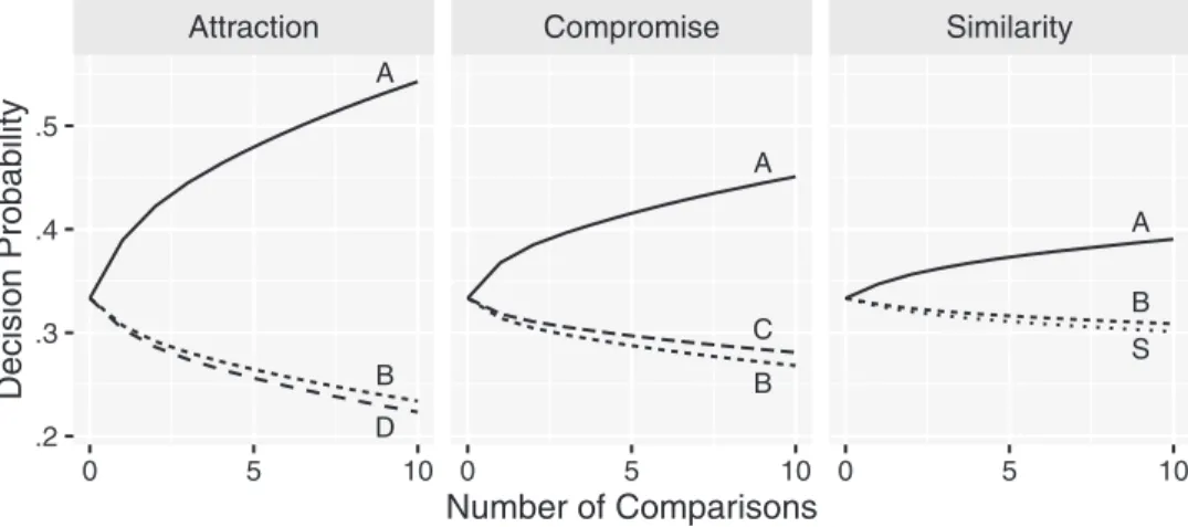
Familiarity with the choice domain reduces strength of the attrac-tion effect (Kim & Hasher, 2005) and the compromise effect (Sheng, Parker, & Nakamoto, 2005). In our application of MDbS model above, the attraction, similarity, and compromise ef-fects emerge purely from the comparisons within the attribute values from the choice set. But in addressing theUngemach et al.’s (2011) supermarket experiment,Stewart et al.’s (2015)attribute distribution

effects, and Walasek and Stewart’s (2015) malleability of loss aversion the effects emerge from the comparison with attribute values from earlier choices, which we assume remain in working memory, or are recalled from long-term memory. The effects of familiarity are also attributed to the sampling of attribute values from long-term memory. It seems quite reasonable to assume that those unfamiliar with the choice domain will have few values to sample from long-term memory, and that experience will provide more values to sample. As more values are sampled from long-term memory, they dilute the effect of the comparisons within the immediate context that were driving the big-three effects, reducing their strength, consistent with the effects of familiarity. To dem-onstrate, we modeled the attribute values in long-term memory with multivariate normal distribution and examined how decision probability changes as more samples are drawn from long-term memory. The results are summarized inFigure 5: As the number of values sampled from long-term memory increases, the big three context effects become weaker.

Time Pressure

Previous studies report that the attraction, compromise, and similarity effects are weaker when a decision is made under time pressure (Pettibone, 2012;Trueblood et al., 2014). This is because under time pressure, people may not have enough time to evaluate each alternative, and a decision tends to be more random (Petti-bone, 2012). We implement this time pressure effect in the MDbS model by limiting the number of pairwise ordinal comparisons made to reach a decision.Figure 6reports these simulations. In the simulations, when two or more cars accumulate the same strength of evidence, one car is randomly chosen. When fewer comparisons are made, decisions are made with less evidence and the big-three effects diminish in size.

Correlations Between the Strengths of the Big Three

Context Effects

Since the specification and initial submission of the MDbS model, we have applied it, unchanged, to new evidence about Figure 4. Effects of varying distance between Car A and the decoy car. The decoy car is located along the gray

the correlations across individuals of the strengths of the big-three context effects. In a meta analysis, Tsetsos, Scheibehenne, Berkowitsch, Rieskamp, and Mata (2017) show the size of the attraction and compromise effects are positively correlated, and that both are negatively correlated with the size of the similarity effect.

These correlations can be explained with variety of mechanisms (Tsetsos et al., 2017). In the MDbS model, one possible way to capture these correlations is via individual differences in the sim-ilarity parameter ␣. To demonstrate, we followedTsetsos et al. (2017)and computed the relative choice share of Alternative A over B while varying the similarity parameter␣from 0 to 5. The MDbS predictions are illustrated inFigure 7, which shows that as the similarity parameter becomes large, the attraction and

compro-mise effects become stronger, but the similarity effect becomes weaker—mimicking the correlations seen in the meta analysis.

A Quantitative Comparison of Closed-Form Models of

the Big Three Context Effects

We have demonstrated that the MDbS model can produce a qualitative account of the big three context effects using one fixed specification of the model with one fixed set of parameter values. In this section we offer a quantitative evaluation of the predictive accuracy of the MDbS model. We use data from a new experiment where participants chose between consumer goods and simultaneously show all of the big three context effects. We compare the predictive accuracy with those of MDFT and MLBA models, two other models designed to cap-Figure 5. Decision probability as a function of the number of attribute values sampled from long-term memory.

Each panel summarizes mean-average decision probability of 5,000 simulations for each number of samples. With the number of samples from long-term memory, the attraction (left panel), compromise (middle panel), and similarity (right panel) effects all become weaker. In this illustration, attribute values in long-term memory are assumed to follow normal distribution whose mean is the attribute values of Car A, and standard deviation is the absolute difference between Cars A and B. We also assumed that attribute values in long-term memory are weakly correlated at Pearson coefficient⫽ ⫺.2. However, the findings of weakened effects with more long-term memory samples are robust across many possible distributions.

ture the big three context effects that also have closed form solutions.

Multialternative Decision Field Theory (MDFT). Decision field theory (Busemeyer & Townsend, 1993) was originally de-veloped to explain decisions between two alternatives but was later extended to explain decisions between more than two alternatives (Roe et al., 2001). MDFT was the first simultaneous account of the attraction, compromise, and similarity effects.

In MDFT, on each time step in the accumulation process, attention is focused on one dimension and attribute value differ-ences are accumulated for all alternatives. In the next time step, attention can switch to a new dimension. During the accumulation process, accumulators are subject to distance-dependent lateral inhibition, where evidence accumulated for one alternative inhibits evidence accumulated for another alternative, and the strength of the inhibition depends on distance between two alternatives in attribute space. The computational implementation of MDFT is described inAppendix D.

The explanation of the similarity effect is similar to that of elimination by aspects. The switching of attention across attribute values means that cars similar in attribute space receive correlated inputs for their accumulators. For example, Cars B and S have positive accumulation when price is attended and negative accu-mulation when fuel efficiency is attended. Car A shows the oppo-site pattern, having positive accumulation when fuel efficiency is attended and negative accumulation when price is attended. This means that Cars B and S tend to have very similar accumulated evidence at each time point and thus end up competing for and sharing wins when price happens to dominate the sampling of attention. Car A however does not have such competition, and so gets all of the wins when fuel efficiency happens to dominate the sampling of attention.

The explanation of the compromise effect is that the distance-dependent lateral inhibition creates a correlation in accumulated evidence between Cars B and C. The logic is as follows. Because the distant dependent inhibition is stronger between the more similar Cars A and C and Cars A and B, the evidence accumulated for these pairs tends to become anticorrelated. If C and B are both anticorrelated with A, then they will become correlated with one another. This means that Cars C and B end up sharing wins—as when one does well so does the other. But Car A does not have to share wins and thus has an advantage.

Finally, the explanation of the attraction effect also depends on distance-dependent lateral inhibition. As Car D is inferior to Car A in both attributes, attribute value differences tend to be negative for Car D, causing the evidence accumulated for Car D to become negative. This negative accumulation, when propagated through the lateral inhibition, gives a positive boost for Car A’s accumu-lator. Car B is sufficiently distant from Car D that Car B’s accumulator is unaffected by inhibition from Car D’s negative accumulation and thus Car B does not receive a boost. Thus only Car A and not Car B is boosted by Car D, and so Car A has the highest decision probability.

This explanation of the attraction effects was criticized as neu-rally implausible because of the reliance upon negative accumu-lator values (Usher & McClelland, 2004), although neurons can drop below threshold levels of firing.Tsetsos, Usher, and Chater (2010)also criticized the account of the attraction effect, pointing out that introducing an extra decoy D’ dominated by Car D should reverse the effect: The worse decoy Car D’ will eventually develop negative evidence, which should lead to boosted accumulation for Car D, which in turn should inhibit accumulation for Car A, creating a reverse attraction effect. Under this reverse attraction effect, Car B is more likely chosen over Car A. It seems improb-able that the addition of another alternative inferior to Car A decreases the probability of Car A being chosen, but this reverse attraction effect has not been empirically examined.

The Multiattribute Linear Ballistic Accumulator (MLBA) model. The linear ballistic accumulator model was originally developed as a simplified model of evidence accumulation (Brown & Heathcote, 2008) but later extended to account for the attraction, compromise, and similarity effects as the MLBA model (True-blood et al., 2014). In the MLBA model, evidence for each alternative is accumulated at a constant but noisy rate. In the MBLA model, the sequential sampling aspect of the accumulation is dropped in favor of a ballistic accumulation process with rates fixed over the duration of the accumulation. The MBLA model also has no assumptions of lateral inhibition between accumula-tors. Instead, the accumulation rate is determined by sum of weighted advantage of an alternative’s subjective values. The subjective value function in the MLBA model favors an alternative with similar attribute values across dimensions. When attribute values range from 0 to 10 on two dimensions, for example, the sum of subjective values for attribute values (5, 5) is higher than that for Figure 7. Correlations between the strengths of the attraction, compromise, and similarity effects over

individuals. A larger value indicates that the effect is stronger, a value of zero indicates that the effect is not predicted, and a negative value indicates that the effect is reversed. The value of␣is indicated with the interior color of dots: white color represents the prediction with␣ ⫽0, and black color represents the predictions with

attribute values (2, 8). In the weighting of advantages, the weight is distance-dependent: a small difference in subjective values is more heavily weighted than a large difference. Further, a disad-vantage is more heavily weighted than an addisad-vantage. The compu-tational implementation of the MLBA model is described in Ap-pendix E.

The explanation of the attraction effect is through the distance-dependent weights on advantages. As a small advantage is more heavily weighted than a large advantage, the advantage of Car A over Car D is more heavily weighted than the advantage of Car B over Cars A or D. As a result, Car A has a higher accumulation rate than Car B. This mechanism is analogous to the distance-dependent lateral inhibition in the MDFT model. Just as the lateral inhibition creates a positive boost only to Car A in the MDFT model, only Car A gains from the presence of Car D in the MLBA model.

The explanation of the similarity effect is through the distance-dependent weights on disadvantages. Only Car A has no small disadvantages— only two large disadvantages to Cars B and S on price. In contrast, Car S has one small disadvantage to Car B on price (the disadvantage to Car A on fuel efficiency is large). Similarly Car B has one small disadvantage to Car S on fuel efficiency (the disadvantage to Car A on fuel efficiency is large). As small disadvantages are heavily weighted, Cars S and B are disadvantaged whereas Car A, which has no small disadvantages, is not. Thus Car A has the highest accumulation rate. Therefore just as Cars B and S inhibit each other in the MDFT model through the distance-dependent lateral inhibition, Cars B and S lower the accumulation rates of each other in the MLBA model through the distance-dependent weights on disadvantage.

For the compromise effect, the cars are more distant from one another. The weight for the medium differences between Cars C and A and Cars A and B is similar to the weight the large differences between Cars C and B. The compromise effect is, instead, explained through different weights on advantages and disadvantages. In particular, Car B’s disadvantage to Car C on fuel efficiency is given more weight than Car B’s advantage over other cars on price. As a result, Car B has a small accumulation rate. Similarly, Car C’s disadvantage to Car B on price is heavily weighted, and thus, Car C has a small accumulation rate. On average, Car A has smaller disadvantages over other cars, and as a result, Car A has the largest accumulation rate. In addition, Car A has a higher subjective value than Cars B and C. This is because the subjective value function requires attribute values to be on the same unit and range across dimensions, and when attribute values are on the same unit and range, Car A has similar attribute values for both dimensions.

The above explanation of the big three context effects stands upon a fine balance between the weights. The MLBA model has been criticized as being too sensitive to small changes in attribute values.Tsetsos, Chater, and Usher (2015), in particular, show that for all of the combinations of reasonable parameter values, it is possible to reverse the attraction effect (i.e., to make Car B preferable over Car A) by introducing small changes to the attri-bute values (see alsoTrueblood, Brown, & Heathcote, 2015). As we describe above, a reverse attraction effect has not been found. Big three consumer choices experiment. To allow us to compare the MDbS, MDFT, and MLBA models on their ability to

capture the big three context effects with consumer choices, we have run a new experiment.

Method. We collected data from 503 participants (204 fe-male, 298 male and 1 undisclosed, whose age ranges from 18 to 75 with the mean of 33) recruited through Amazon Mechanical Turk (https://www.mturk.com). Each participant was paid $1.00 for taking part.

We asked each participant to make eight decisions in a random order: two control decisions between three alternatives, where one alternative dominates the other two; three decisions between three alternatives, each of which was intended to invoke the attraction, compromise and similarity effects; and three decisions between two alternatives. Each alternative was described in terms of two dimensions. Two or three alternatives were displayed in a table, and the participants made decisions by clicking on an alternative. In the table, attribute dimensions were organized in rows, and alternatives were organized in columns. The order of columns (e.g., which alternative to appear on the left column) and the order of dimensions (e.g., which dimension to appear on the first row) was randomly shuffled for each participant for each trial.

The decisions in the experiment were between various consumer products. We prepared eight consumer product cover stories (e.g., mouthwash, and boxes of chocolate; see Appendix F for the complete list). Each cover story contained two alternatives, and these alternatives were presented to participants for the two-alternative decisions. For the three-two-alternative decisions, we ran-domly selected one of the two alternatives and generated a third alternative in a way that the context favors the selected alternative. To generate a third alternative for an attraction choice, for example, we first calculated the absolute differences between Alternatives A’s and B’s attribute values on each dimension. To create an attraction choice which favors Alternative A, we gener-ated AlternativeDA by subtracting 25% of the differences from

Alternative A’s attribute values, so that AlternativeDAis inferior

to Alternative A in both dimensions. To create AlternativeDB, we

subtracted the same 25% from Alternative B’s attribute values. To generate a third alternative for a similarity choice to favor Alter-native A, similarly, we subtracted 2% of the A-B difference from Alternative B’s attribute value on one dimension and added 2% of the A-B difference to Alternative B’s attribute value on the other dimension.

As a result, each cover story has two versions of choice sets for each of attraction, compromise, and similarity effects: one whose context favors Alternative A and the other whose context favors Alternative B.

We decided, in advance of data collection, to recruit 500 par-ticipants and remove the data collected from the parpar-ticipants who choose a dominated alternative in either or both of the control choices.

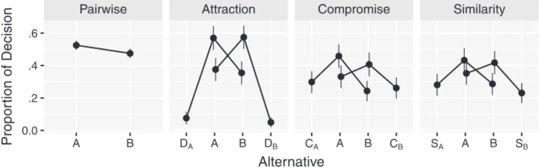
compromise and similarity effects: Alternative A is most often chosen, when the third alternative (DA,CA, orSA) was positioned

in a way intended to favor Alternative A under the expectation of replicating the attraction, compromise and similarity effects. In contrast, when the third alternative (DB,CB, orSB) was positioned

in a way intended to favor Alternative B, Alternative B was most often chosen.

Although the attribute values in the experiment have different scales and units, the MDFT and MLBA models require attribute values to be on the same scale and unit. Thus for the MDFT and MLBA models, we linearly transformed attribute values, such that Alternative A always had attribute values (3, 2) and Alternative B had attribute values (2, 3).

In fitting the models, we used a hierarchical Bayes framework. This framework allows parameter values to vary between partici-pants but also pulls parameter values toward estimates at the group level (seeAppendix Hfor more details and estimated parameter values). Thus, hierarchical Bayes allows the strengths of the con-text effects to vary between participants, which has been previ-ously reported (Berkowitsch, Scheibehenne, & Rieskamp, 2014; Tsetsos et al., 2017).

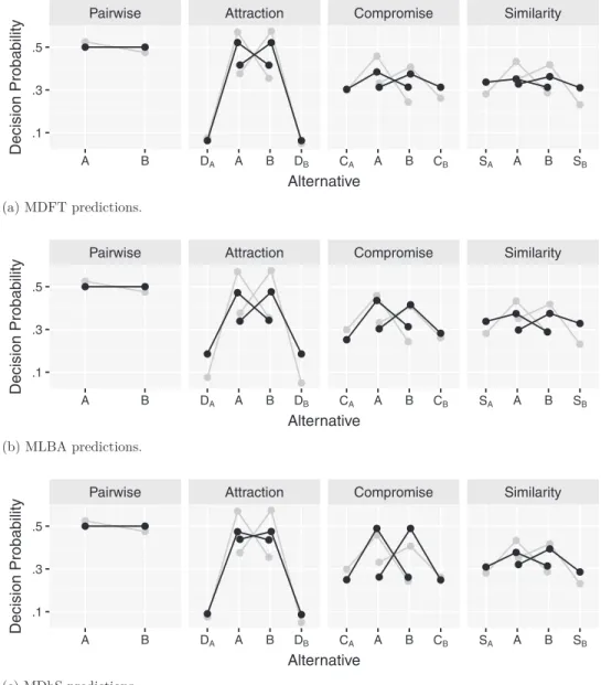
With the parameter values estimated at the group level, we made predictions on the data with the three models. The results are summarized inFigure 9, which shows that the three models pro-duce the qualitative patterns of context effects. Compared with the observed proportion of decisions (gray dots replicated from Figure 8), the MDFT model predicts strength of attraction effect quite well but tends to underestimate the similarity and mise effects. The MLBA model, in contrast, predicts the compro-mise effect well but underestimates the attraction effect and, to a lesser extent, the similarity effect. Finally, the MDbS model pre-dicts the compromise effect well but underestimates the attraction effect and, to a lesser extent, the similarity effect. Overall, how-ever, none of the models appears to provide superior predictions across the three effects.

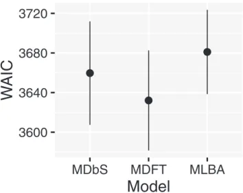
The performance of each model was quantitatively assessed with the widely applicable information criteria (WAIC;Watanabe, 2013; see also, Gelman, Hwang, & Vehtari, 2014). By using WAIC, we assess out-of-sample predictive accuracy: a model is favored if the model makes a better prediction for a new data point. An alternative approach, which we did not take, is to assess

in-sample error: a model is favored if the model provides a better fit to the data we collected. This alternative approach often relies on BIC or Bayes factor (please seeGelman et al., 2013, for more discussion on the two approaches). WAIC is an estimate of ex-pected predictive accuracy, and smaller values indicate that a model’s prediction for a new observation is likely to be more accurate. Thus, WAIC is larger for a model which over- or under-fits the data. The results are summarized inFigure 10.Figure 10 shows overlapping error bars, indicating that in terms of performance, the MDFT, MLBA, and MDbS models are not distinguishable. One advantage for MDbS model is that it does not require attribute values to be on the same scale and unit, but can still achieve performance comparable with the MLBA and MDFT models.

Thus far, we have seen that the MDbS model can provide an account of the big three context effects. The mechanisms in the MDbS model were constrained by eye movement process data, but MDbS generalized well to choice proportions for the big-three choice phenomena. In fact, despite— or perhaps because of—these constraints, MDbS’s quantitative account is about the same as that offered by other the prominent accounts from the MDFT and MLBA models. Below we turn to the additional multialternative decision phenomena in the literature and consider the breadth of accounts offered by the MDbS, MDFT, MLBA, and componential context models.

A Qualitative Account of the Breadth of

Multialternative Decision Phenomena

In this section, we compare the models in their capabilities to explain a broad range of multialternative decision phenomena beyond the big three context effects. To identify other key phe-nomena, we surveyed theoretical studies which discuss at least two of big three context effects. All of the phenomena discussed in these studies are listed in Table 3. ThusTable 3 represents the range of phenomena of concern in the literature, and not a hand-picked list of phenomena that the MDbS model can explain. The first three rows concern experiments run by Stewart and colleagues which we have described above. The remaining rows are about experiments run by other researchers. We note in the main text and the footnotes toTable 4where minor modifications might be made Figure 8. Choice proportions for each alternative in the big-three consumer choices experiment. Each panel

to theories to capture effects— otherwise, effects are captured by the “vanilla” models as presented here without any modification. With these choice sets, we examined whether a model explains the context effects by testing all of the possible combinations of reasonable parameter values (seeAppendix J for more details). Then, we examined the maximum number of context effects a model can explain. Given the purpose of the existing models, we restrict our attention to the parameter values which produce the attraction and compromise effects for the componential context model (discussed below) and the attraction, compromise and sim-ilarity effects for the MDFT and the MLBA model.

As with the quantitative comparison above, we normalized the attribute values for all models, except the MDbS model which does not require this. The normalized attribute values are listed inTable J1inAppendix J.

Below we describe the modeling of each phenomenon in detail. We have reused the single set of MDbS parameter values from

earlier:␣ ⫽3.0, ␤₀⫽ 0.1,␤₁ ⫽50, and␪ ⫽0.1. Overall, the results highlight that the MDbS model predicts a wider range of context effects than the existing models. First though, we introduce the componential context model and briefly review other models. The componential context model. We have included the componential context model (CCM;Tversky & Simonson, 1993) in the qualitative evaluation. We omitted it from the quantitative evaluation of the big three effects because the model does not account for the similarity effect (Roe et al., 2001) and because the model does not produce decision probabilities. The CCM was developed to explain the background contrast and the compromise effects. In the CCM, the subjective value of an alternative is an average of two quantities: a weighted sum of attribute values, which explains the background contrast effect; and a relative advantage of attribute values, which explains the attraction and compromise effects. The CCM produces subjective values for each alternative, and the alternative with the highest subjective value is Figure 9. Mean predictions for the big-three consumer choices experiment, with the parameter estimates at the

chosen. Thus, unlike the other models we have discussed, the CCM does not implement an evidence accumulation process. As a result, the CCM does not explain the effects associated with time pressure. Previously,Soltani et al. (2012)simplified the CCM and show that the CCM predicts a stronger attraction effect with a closer decoy, but without the simplification, the CCM correctly predicts a weaker attraction effect with a closer decoy. The com-putational implementation of the CCM is described inAppendix I. Other models. Other evidence accumulation models often require simulations to produce predictions. One simulation run of such model produces one decision. It takes of the order of 1,000 or more simulation runs to estimate decision probabilities with suf-ficient precision. Such models include the leaky competing accu-mulator model (Usher & McClelland, 2004) and the associative accumulation model (Bhatia, 2013). Other models, which this article does not review, include 2N-ary choice tree model (Wollschläger & Diederich, 2012) and range-normalization model (Soltani et al., 2012).

The Alignability Effect

In the alignability effect, attributes that are shared over alternatives have a greater impact on decisions and valuations than attributes that are unique to single alternatives (Markman & Medin, 1995;Slovic & MacPhillamy, 1974;Zhang & Markman, 2001). For example, con-sider a choice between two microwave popcorns. Popcorn A is described in terms of calorie content and kernel size, and Popcorn B is described in terms of calorie content and sweetness of taste. The common calorie content attribute has greater impact on decisions than the unique kernel size and sweetness attributes.

The alignability effect has been explained with the notion of ease of comparison. A comparison between alternatives along the common dimension is considered cognitively easier, and this ease of comparison is considered to lead to greater reliance on the common dimension (Slovic & MacPhillamy, 1974).

In the MDbS model, this ease of comparison is related to the difference between attribute values that are already in working memory because they are part of the problem and attribute values that must be sampled from long-term memory. In the above example, a comparison on calories is relatively likely, because calorie values are available in working memory for both alterna-tives. In contrast, when evaluating alternatives on noncommon dimensions, people must sample relevant values from long-term memory, but people do not appear to always do this sampling from long-term memory (e.g.,Kassam, Morewedge, Gilbert, & Wilson, 2011). People’s working memory, for example, may be already fully loaded with attribute values sampled from other alternatives in the choice set. Without sampling from long-term memory, the noncommon attributes will not be used in comparisons and will not contribute to the accumulation rates.

Further, there will be individual differences in the sampling. When evaluating popcorn’s sweetness, for example, some people may sample the extreme sweetnesses of candies from long-term memory, whereas others may sample the more subtle sweetness in fruits. Thus for some people the popcorn’s sweetness will be evaluated favorably and for others it will be evaluated unfavorably. Consequently, when averaged across people, attribute values on noncommon dimensions will not appear to explain people’s valu-ation and decisions.

The Attribute Balance Effect

The attribute balance effect is found when two attribute dimensions are on the same scale range and unit. An example is when available cars are rated on the scale from 0 to 100 for both warranty and fuel efficiency (see the left panel inFigure 11). Under this condition, people tend to decide on an alternative which has the same ratings for both attributes (Chernev, 2004, 2005).

This attribute balance effect has been attributed to people’s aversion to disperse values within an alternative (Chernev, 2005). For example, the attribute values for Car L in the left panel ofFigure 11differ from each other by 20⫽70 (efficiency rating) – 50 (warranty rating). This difference is considered to reduce the attractiveness of Car L. Thus, this account postulates that people collapse the attribute dimensions and compare at-tribute values across dimensions. In support, Chernev (2004) reports that when participants were primed to examine alterna-tives attribute by attribute and not to collapse the dimensions, their decisions do not show the attribute balance effect. In addition, when the attribute dimensions are not collapseable (e.g., because of different units), the attribute-balance effect is not observed (Chernev, 2004).

The MDbS model explains the attribute balance effect by al-lowing people to compare values across attribute dimensions when attribute dimensions are commensurable. The efficiency rating of Car L, for example, may be compared against the warranty rating of Car Q. When attribute dimensions are collapsed, the balanced alternative (i.e., Car Q) becomes the compromise alternative. In a choice set with Cars K, L, and Q inFigure 11, the attribute values after collapsing the dimensions are {40, 50, 60, 60, 70, 80}. The middle two values, 60, belong to Car L. Then, the attribute-balance effect emerges with the same mechanism as the compromise Figure 10. Model performance measured with the widely applicable