Audio visual olfactory resource allocation for tri modal virtual environments

warwick.ac.uk/lib-publications

Manuscript version: Author’s Accepted Manuscript

The version presented in WRAP is the author’s accepted manuscript and may differ from the

published version or Version of Record.

Persistent WRAP URL:

http://wrap.warwick.ac.uk/114490

How to cite:

Please refer to published version for the most recent bibliographic citation information.

If a published version is known of, the repository item page linked to above, will contain

details on accessing it.

Copyright and reuse:

The Warwick Research Archive Portal (WRAP) makes this work by researchers of the

University of Warwick available open access under the following conditions.

Copyright © and all moral rights to the version of the paper presented here belong to the

individual author(s) and/or other copyright owners. To the extent reasonable and

practicable the material made available in WRAP has been checked for eligibility before

being made available.

Copies of full items can be used for personal research or study, educational, or not-for-profit

purposes without prior permission or charge. Provided that the authors, title and full

bibliographic details are credited, a hyperlink and/or URL is given for the original metadata

page and the content is not changed in any way.

Publisher’s statement:

Please refer to the repository item page, publisher’s statement section, for further

information.

Audio-Visual-Olfactory Resource Allocation for Tri-modal Virtual

Environments

E. Doukakis, K. Debattista, T. Bashford-Rogers, A. Dhokia, A. Asadipour, A. Chalmers, and C. Harvey

Abstract—Virtual Environments (VEs) provide the opportunity to simulate a wide range of applications, from training to entertainment, in a safe and controlled manner. For applications which require realistic representations of real world environments, the VEs need to provide multiple, physically accurate sensory stimuli. However, simulating all the senses that comprise the human sensory system (HSS) is a task that requires significant computational resources. Since it is intractable to deliver all senses at the highest quality, we propose a resource distribution scheme in order to achieve an optimal perceptual experience within the given computational budgets. This paper investigates resource balancing for multi-modal scenarios composed of aural, visual and olfactory stimuli. Three experimental studies were conducted. The first experiment identified perceptual boundaries for olfactory computation. In the second experiment, participants (N=25) were asked, across a fixed number of budgets (M=5), to identify what they perceived to be the best visual, acoustic and olfactory stimulus quality for a given computational budget. Results demonstrate that participants tend to prioritize visual quality compared to other sensory stimuli. However, as the budget size is increased, users prefer a balanced distribution of resources with an increased preference for having smell impulses in the VE. Based on the collected data, a quality prediction model is proposed and its accuracy is validated against previously unused budgets and an untested scenario in a third and final experiment.

Index Terms—Multi-Modal, Cross-Modal, Tri-Modal, Sound, Graphics, Olfactory

1 INTRODUCTION

The existence of multiple stimuli in a VE is required for increasing immersion in many current and future applications. The inclusion of realistic olfactory delivery along with audio-visual stimuli is of key importance if VEs are to be used as genuine representations of real life scenarios [36]. The introduction of smell impulses increases the sense of presence in the virtual world and enhances the level of realism [16]. The significance of a tri-modal combination of smell, vision, and hearing might not be initially obvious but it affects how people think, feel and behave [40].

Accurate computation and delivery of multiple stimuli in high fi-delity requires significant computing capability. Previous research has shown that humans cannot fully attend to all the incoming sensory stim-uli in the real environment. Such cross-modal interaction phenomena and known limitations of the HSS have been utilized to reduce compu-tational requirements [29] without the users being able to perceive any quality degradations. Furthermore, it is unclear how best to allocate computational resources in a VE. For example, if an improvement in computational performance of 50% becomes available, how would it be best to make use of that extra computational power. Is it best spent on improving visuals? Improving the audio? A smaller improvement to both? Adding smell? Resource allocation schemes have been recently proposed to describe distribution of available resources based on human subjective preferences [19]. However, previous work is limited to two modalities, in particular, audio and vision.

The work presented in this paper captures how human allocation preferences are adjusted given a budget of computational resources in a tri-modal VE set up. In order to establish how this computational budget can be distributed between the three senses, three experiments have been conducted. Experiment I was focused on understanding the perceptual limitations of olfactory computation, such that the

compu-• Correspondence to E.Doukakis, [email protected] or K.Debattista, [email protected]

• E. Doukakis, K. Debattista, A. Dhokia, A. Asadipour and A. Chalmers are with University of Warwick

• T. Bashford-Rogers is with University of the West of England • C.Harvey is with Birmingham City University

Manuscript received xx xxx. 201x; accepted xx xxx. 201x. Date of Publication xx xxx. 201x; date of current version xx xxx. 201x. For information on obtaining reprints of this article, please send e-mail to: [email protected]. Digital Object Identifier: xx.xxxx/TVCG.201x.xxxxxxx

tational requirements for olfactory delivery can be established. With this knowledge, Experiment II was conducted whereby participants allocated computational resources across visual, auditory and olfactory stimuli in order to identify a perceptually optimal load balancing of these resources from a given fixed budget. This was conducted at five different computational budgets for a number of scenarios. Based on the collected subjective data, a resource distribution model is proposed and evaluated on untested budget sizes and scenarios in Experiment III. Therefore, multi-sensory rendering pipelines can exploit such a model to direct resource allocation decisions in VEs.

The main contributions of this work are as follows:

• A psychophysics framework for estimating odour just noticeable difference (JND) thresholds for a range of smell concentration magnitudes.

• An experimental methodology for allocating resources in tri-modal VEs.

• Evidence that participants generally prefer to allocate resources for visual stimuli. However, as the budget increases the percent-age devoted for aural and olfactory stimuli in the virtual scenario is increased significantly.

• A validated model capable of predicting resource allocation in systems where visual-aural and olfactory cues are intended for delivery.

2 BACKGROUND ANDRELATEDWORK

Simulation and delivery of multiple senses at the same time is consid-ered crucial for ensuring a realistic experience and increase a user’s overall level of immersion [21]. Applications of multi-sensory VEs range across different sectors of academia and industry. In reality, per-ceiving one sensory stimulus is quite rare in the physical world and many studies that investigate multiple senses, have found that the per-ceptual impact of one sense to the other can be quite significant [5, 20].

2.1 Audio-Visual Interactions

better visuals decreased the perception of quality in the acoustic domain.

This effect was shown to be practical by Moecket al.by using

hierar-chical clustering of sound sources given congruent visual signals [34]. Perceptual interactions as triggered by sound cues are explored by Rocchesso [13]. Using sound effects, a series of human-human and human-object interactions are explained and validated. Preserving the

level of presence in a VE has recently been examined by Graniet al.[8].

In their work, audio-visual attractors are used in an experimental study to quantify how users’ attention is directed in a cave automatic virtual environment, avoiding gaps in presence. Sound has also been shown to influence perception in the spatial domain, such that congruent sounds can direct attention. This effect has been used in selective rendering models [26].

2.2 Olfactory-Visual Interactions

Olfactory-visual stimulation has been shown to increase presence in both generalized virtual environments and in targeted virtual environ-ments when compared to a visual only condition [18, 35].

Supple-mentary to this, Munyanet al.[35], showed that when the olfaction

condition was removed, this resulted in a disproportionate decrease in presence. Attentional changes have been observed when humans are presented with multi-sensory stimuli when compared to a visual only

condition. Seoet al.[42] observed congruent objects impacting

view-ing time and deviatview-ing eye fixation. Seignuricet al.[41] investigated

the influence ofa-prioriconnections in between a scent and congruent

visual stimuli on eye saccades and fixations, showing that congruent

ob-jects were explored faster in the presence of the odour. Chenet al.[15]

performed a study to corroborate this effect and concluded that a multi-modal saliency map weighing both visual and olfactory inputs was

required. Harveyet al.[25] showed that conventional image saliency

maps can no longer be relied upon in the same way in olfactory-visual environments and demonstrated a validated model based on empirical findings.

2.3 Multisensory Integration

Burr and Allais have proposed a linear model for bimodal fusion in the audio-visual domain [6]. This suggests that weights control the bimodal

information from the two senses: ˆS=wASˆA+wVSˆV, wherewAand

wV scale the estimates for audio and vision respectively, ˆSAand ˆSV.

Multisensory VEs are computationally demanding when considering the simulation of numerous senses [22]. It is however possible to balance computation to account for the weight that the human sensory system places on each sense. However, multisensory VEs have inherent perceptual affects that have to be understood [4], before these weights

can be derived. In the study proposed by Doukakiset al.[19], the

authors presented a method for resource allocation in bi-modal VEs, namely vision and hearing, based on human subjective preferences. In that experimental study, participants allocated a given budget of resources to improve the quality of the audio-visual stimuli. Based on the results, an estimation model is proposed and validated. Similar

methods have been used by Slateret al.[14] to investigate the level

of presence in VEs by conducting experiments where experienced participants at immersive system methodologies vary four possible graphical factors. In a subsequent experimental study by Skarbez

et al.[12], participants could adjust a series of coherence factors to increase the level of the plausibility illusion, to match the perceptual experience they had in a highest coherence scenario. Results showed that participants prioritize improvements to the virtual body.

Ernst and Banks [11] investigated which of the senses of vision and haptics is more dominant using a maximum-likelihood estimation on the combined input of both sensory cues. Using the variances of each sense in height estimation, a maximum-likelihood integrator model is given and compared to human collected data in visual-haptic

tasks. Azevedoet al.[7] considered how the senses of vision, hearing,

olfactory and haptics are classified for measuring presence, focusing on outdoor VEs. Their results showed that the combined effect of haptics and hearing was considered more important than the typical VE stimuli of vision and hearing, dependent on scene and plausibility illusions.

In summary, there exists a large body of work that considers the permutations of senses and their respective influences on human per-ception and presence. Studies that consider multisensory integration are shown to be of benefit in VEs when resources are adapted based upon empirical findings. In the bi-modal case, this resource allocation has been quantified but beyond remains unexplored.

3 MOTIVATION ANDOVERVIEW

In this work, we are interested in identifying how to best allocate computational resources across audio, vision and olfaction. While audio and vision are reasonably well understood and have been used in a significant number of cross-modal experiments [29], this is not the case with olfaction. Following the audio-visual approach of Doukakis et al. [19], our tri-modal model is built around permitting users to adjust the required computation for all the senses to fit within a given computational budget. The selection and adjustment of the aural and visual stimuli is based on the approach adopted by Doukakis et al. [19]. However, since the application of olfaction in virtual environments is less understood, our initial experiment (Experiment I, Section 4) seeks to identify a useful perceptual parameterization for olfactory stimuli. Experiment II (Section 5) then collects data for load balancing across the tri-modal stimuli at five budgets across three scenarios. Section 6 uses these results to develop a model for tri-modal resource allocation. Finally, Experiment III (Section 7) validates the model.

4 EXPERIMENTI: IDENTIFYING OLFACTORY PARAMETERS

This section describes the olfactory simulation and its parametrisation. Olfaction will be parameterized by the mesh size (as we are using a finite element solver) as it effects the convergence rate of our olfactory simulation using computational fluid dynamics (CFD). An experimen-tal framework is then described for estimating JNDs in a range of concentration magnitudes. The JND threshold estimation allows us to assess whether the recorded concentration curves for different mesh discretization levels are perceptually equivalent. As shall be shown, simulations across a wide range of mesh parameterizations (from 1K to 1M) are not perceptually noticeable by human observers.

4.1 Simulation

This section presents the framework used for simulating smell transport in four test VEs, as shown in Figure 1, using CFD. Odour concentration is captured at virtual probes during the simulation stage across a range of different quality meshes. In this work, the considered mixture is composed by the smell of citral in air and the objective is to estimate the concentration of citral during the transport of the mixture.

All the CFD simulations were implemented using theEulerian

ap-proach, i.e. compute the variables of interest over time at the centres of the control volumes (CVs) that compose the domain’s computa-tional mesh. This procedure requires two steps. Firstly, it includes the discretisation and solution of the Navier-Stokes equations that gov-ern the transport of the air-odour mixture and compute its momentum

(−→U), pressure (p) and density (ρ). Secondly, coupling the governing

equations with a transport differential equation for estimating the

con-centration of the odour, denoted asC, at every node of the mesh. This

equation is of the general form:

∂ ρC ∂t | {z }

temporal term

+ ∇·(ρ−→U C)

| {z }

convection term

− ∇·−→J | {z }

diffusion term

= SC(C)

| {z }

source term

, (1)

where the quantity−→J =ρDca∇C)is the mass diffusion flux of the

odour andDca=8.23×10−5m2/s is the diffusion coefficient of citral

into the air [33]. The termSC(C)describes the effect of body forces

and is used to model the effect of the Earth’s gravitational field. The temporal term and the terms that model the physical processes of convection and diffusion are underlined in Equation 1. As is the case with every odorous gas, the flow transport of the citral-air mixture is highly turbulent. Turbulence effects were implemented using a

Fig. 1. The boundary conditions of the VEs used at this experimental study, From left to right: Bathroom interior, Car, Kitti, Kitchen. The blue painted patches represent the odour inlets while the red patches are used for developing convention effects. The green coloured spheres represent the virtual probes for reading concentration values.

The domain’s mesh granularity affects the solution’s convergence rate while it can increase numerical stability during the simulation [39]. Coarse meshes yield concentration solutions with over- and undershoots because of the non-smooth transition of the odour-air mixture across the CVs. We considered four different mesh versions of successively higher number of CVs for every one of the three scenarios. These are meshes with 1K, 10K, 100K and 1 million CVs. The coarsest mesh was refined near the surfaces and the boundaries of the VE for better accuracy while every successive refinement was uniform across the domain so as to approximately preserve the initial distribution of CVs in the boundaries. Mesh sizes with an order of magnitude change in the number of CVs were selected in order to study how odour concentration at probe locations changes between large spatial discretisation steps starting from very coarse up to excessively high refinement levels.

4.1.1 Application to VEs

Simulation of smell propagation was considered in four different VEs. These are depicted in Figure 1. All the physical quantities used as boundary conditions were obtained by measuring concentration and flow rate with a photoionization detector and a flow meter respectively in the real places that were used for creating the VEs. The final values resulted through averaging of the results collected over 10 repeated measurements. These scenarios were chosen because the convection process occurs in a different way in each scenario, and therefore the smell will be dispersed differently. In the Bathroom, temperature

differ-ences between the hot bath (45oC) and the environment (15oC) cause

the smell-air mixture to circulate in the room. In the car scenario, con-vection is simply created due to the air flow coming through the vents

at a constant temperature of 25o_{C. In the Kitti scenario, convection}

occurs due to the air coming through the three doors. In the Kitchen scenario, convection effects are introduced through the temperature

gradient between the hot kettle (50◦C) and the cold environment (15

◦_{C). Pressure was assumed to be the same and equal to atmospheric}

pressure (101.325 Pa) for all three VEs. Figure 1 depicts the smell inlet

boundaries and the patches used for developing convection effects in the VEs. The same figure also shows the locations of the virtual probes in the VEs.

4.1.2 Smell concentration results

Smell concentration values were recorded at the virtual probe using a sampling frequency of 4Hz. This sampling rate was chosen based on the rate many photoionisation devices record odour concentration values in real environments [23].

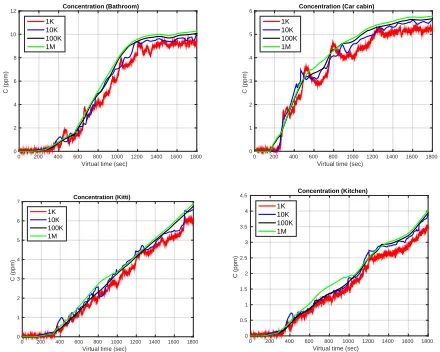
For all the VEs, smell propagation was simulated for 1,800 seconds

of virtual time to see how concentration evolves at the sensor location for a sufficient amount of time. Figure 2 shows how concentration changes over time for the four different spatial discretisation levels. For coarse meshes the transition of the air-citral mixture near the sensor position is more abrupt therefore fluctuations are captured in the con-centration function. These fluctuations are progressively eliminated as the mesh is refined. As can be seen from the graphs in Figure 2, the con-centration curves are not very distant from each other. Specifically, the maximum difference between the coarsest (1K) and the finest meshes

(1M) was 1.98 ppm for the Bathroom scenario, 1.623 ppm for the Car

scenario and 1.345 ppm for the Kitti scenario. Furthermore, the curves

stabilise as the VE becomes saturated from the emitted odour. After this equilibrium point, concentration does not change significantly. The equilibrium point has not been fully achieved for the Kitti scenario

because of the large volume of the room (560.64 m3) and the location

of the sensor.

Virtual time (sec)

0 200 400 600 800 1000 12001400 1600 1800

C (ppm)

0 2 4 6 8 10

12 Concentration (Bathroom)

1K 10K 100K 1M

Virtual time (sec)

0 200 400 600 800 1000 1200 1400 1600 1800

C (ppm)

0 1 2 3 4 5

6 Concentration (Car cabin)

1K 10K 100K 1M

Virtual time (sec)

0 200 400 600 800 1000120014001600 1800

C (ppm)

0 1 2 3 4 5 6

7 Concentration (Kitti)

1K 10K 100K 1M

Virtual time (sec)

0 200 400 600 800 1000 1200 1400 16001800

C (ppm)

0 0.5 1 1.5 2 2.5 3 3.5 4

4.5 Concentration (Kitchen)

1K 10K 100K 1M

Fig. 2. Concentration results measured for different mesh discretisation levels at the virtual probe locations. Top-left: Bathroom, Top-right: Car, Bottom-Left: Kitti, Bottom-Right:Kitchen.

4.2 Method

In this study the experimental methodology used for estimating the JND threshold was the two interval forced choice (2IFC) method [30]. At every trial two olfactory stimuli were presented with an interstimulus time interval (ITI) between them. The first is a constant concentration stimulus, known as a pedestal, while the second is a varying stimulus randomly selected from a predefined set of concentration magnitudes. Ten trials were implemented for each comparison pair (pedestal, vary-ing) for the different values of the varying stimulus. The presentation order of the two smell impulses (pedestal-varying or varying-pedestal) was also randomized across the experimental trials to avoid any poten-tial ordering bias.

The JND threshold is the magnitude that needs to be added to the pedestal so as the resulting olfactory stimulation has a magnitude that is perceptually more intense than the pedestal in 75% of the total trials [30]. During each trial, the two stimuli were presented with an ITI interval of 4 seconds while the stimulus exposure duration (SED)

was 0.5 seconds for each of the two delivered bursts. A short SED was

selected to avoid user adaptation to the released smell while the ITI was sufficiently long to permit the participants to rest before inhaling the second stimulus.

while it contains two digital mass flow controllers (DMFCs) for ad-justing the flow rate of each channel as a proportion of the maximum flow rate provided which is 1000 ml/min. For our olfactory display, the suggested operating range for guaranteed concentration accuracy of

the delivered stimulus isI= [C0,Cmax] = [1.2,11.2], parts per million

(ppm) for a SED time of 0.5 sec. All the participants were able to detect

the lemon like odour when they sniffedC0, thus, the whole range of

stimuli contained inIwere higher than the absolute detection threshold.

As there was no previous knowledge for the existence of any JND

threshold in the rangeI, starting withC0 as the pedestal, pairwise

comparisons ofC0with a number of varying stimuli that uniformly

discretizeIwere planned until the average performance among all the

participants would reach a proportion of 75%. For a stepsthe interval

Iwas subdivided to three mutually exclusive subsets:

I1= [1.2+s,1.2+2s,· · ·,1.2+8s]

I2= [4.8+s,4.8+2s,· · ·,4.8+8s]

I3= [8+s,8+2s,· · ·,8+8s].

(2)

A step sizes equal to 0.4 was selected so as to keep a reasonable

number of varying stimuli for each of the three subintervals and be able to span the whole range in the extreme case that no

perceptu-ally different magnitude existed betweenC0and any of the stimuli in

I1,I2,I3. Starting with comparisons of the pedestalC0with the stimuli

in intervalI1, if there was no stimulus that triggers a perceptual

dif-ference, denoted asC1the experimentation would be carrying on in a

subsequent experimental session for the same pedestal and the stimuli

with magnitudes in the intervalI2until the first stimulus that triggers a

perceptual difference. If there was no such stimulus, the pedestal would

be compared with stimuli inI3. In caseC1could be found, there is no

need to continue experimenting for the rest of the stimuli in any of the

I2and/orI3as it was necessary to find perceptual differences starting

fromC1as the new pedestal.

The first time that a JND threshold was found a new experimental session was initiated by adjusting the step for spanning the rest of the

intervalIusing Weber’s law. This law has been applied in the olfactory

domain [3] and states that the ratio of the JND to the pedestal stimulus is constant. Specifically:

JND

Cp

=Cf−Cp

Cp

=k, (3)

whereCpis the pedestal andCf the final intensity stimulus that triggers

a perceptual difference. The constantkcan be obtained from the first

JND, denoted as JND1, and the first pedestalC0=1.20 ppm. Using

the constantk, we can obtain an estimation of the final stimulus that

elicits a perceptual difference starting fromC1as the new pedestal and

applying again Weber’s law. In case the estimation is not in the interval

I, no further experimentation is required as it cannot be delivered by

the olfactory display. If not, a subinterval with a new discretization step is derived and a new experimental session is initiated. The new subinterval includes Weber’s law estimation as the potential stimulus that elicits perceptual difference. The new step is computed so as the new interval does not exceed 10 varying concentration magnitudes.

This adaptive method allowed us to speed up the process of finding a new stimulus that triggers a perceptual difference without comparing intermediate pairs that would be perceptually similar using the initial

small step of 0.4. The derivation of a new step enabled avoiding

unnecessary experimental trials. Using this methodology, two JND

thresholds were found in the operating rangeI. The first one was

included inI1while the second one was found after one step adjustment

using an interval of 10 varying stimuli.

4.2.1 Materials

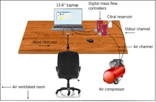
For this study a 15.600laptop computer was used for controlling the

olfactory display and the graphical user interface (GUI). The apparatus is shown schematically in Figure 3. Two tubes arrived near the nose from the olfactometer, one that delivered smell bursts at every exper-imental trial and one air control channel that was evacuating the old

smell stimuli by releasing humidified air at an exact flow rate of 1000 mL/min during the ITI.

Fig. 3. Experimental set up for Experiment I.

The distance of the nose away from the smell delivery point was kept constant at 7 cm using a chin rest located in front of the laptop. An air compressor located under the table was used to provide two air channels for the experiment at a constant pressure of 2 Bars. The first channel was aromatized by passing through a smell reservoir where citral in liquid form was stored. Both the aromatized and the control channel were controlled using the DMFCs which were connected through USB ports on the laptop.

The odour of citral was used as the delivered olfactory stimulus in this experimental study. This is a frequently encountered volatile organic compound (VOC) reminiscent of the smell of lemon. Citral has a low detection threshold that ranges between 25 to 350 ppb [2]. All the participants were able to detect it and no participant reported the smell

as unpleasant. The rangeIcontained intensity stimulations that varied

from faint up to more intense smell impulses without being irritating for the people who smelled them. The experimentation procedure was conducted under normal indoor lighting conditions in a room where air was constantly ventilated during the 4 days of conducting the experiment.

4.2.2 Participants and Procedure

Two groups of 10 participants (11m, 9f, age range 19 to 35,µ= 31.6)

from various academic and working disciplines. The average age of all

the participants was 31.6 years old. No participant reported olfactory

deficits or temporary/permanent anosmia problems.

For each trial, every participant had to smell the two bursts and then decide which one was the most intense by pressing one of the GUI

buttons provided. During the tutorial session, pairs of(C0,C0)stimuli

were presented and the participant was asked if the smell was familiar or not. All the 20 participants were able to recognize the delivered odour. Participants were presented smells with the GUI providing context of the order and the participant could select the most intense stimulus from the GUI. Subsequently, the participant was permitted to select next, at their leisure, to continue onto the next trial. In the first phase each participant conducted eight trials and in the second they conducted ten trials.

4.2.3 JND Results

Two JNDs were found in the operating rangeIprovided by the olfactory

display at two different experimentation phases. The first estimated stimulus that elicited a perceptual difference had magnitude in the

subintervalI1while the second was obtained using one step adjustment

with the adaptive method described previously.

Phase 1 started with a pedestal stimulusC0=1.20 ppm while there

were 8 varying stimuli to compare it with (seeI1interval at Equation 2).

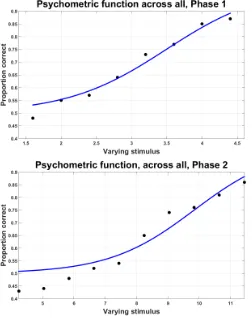
Figure 4 depicts the proportion of correct answers across all 10 partici-pants participated in this phase and the Logistic Psychometric function (PF) fitted to the data. This function was preferred over others as it most accurately fitted the obtained data using deviance criterion as a model comparison metric [30]. For the 2IFC method, the stimulus that corresponds to 75% of correct answers is given through the PF and

corresponds to the magnitudeC1=3.50 ppm. Therefore, the first JND

Fig. 4. Proportion of correct answers across all participants in Phase 1(Top) and Phase2(Bottom). The blue colored curve is the Logistic Psychometric function fitted to the data in both cases.

The slope of the PF expresses how participants’ performance changes with increasing concentration magnitudes. The estimate for

this value wasS1=0.14 units of performance per ppm. The standard

error for the PF estimates forC1andS1were obtained based on a

parametric bootstrap analysis forN=1000 generated data sets using

the collected data of phase 1. For all the generated data collections the

parametersC1andS1were estimated and their standard deviation was

computed. These were SDC1=0.12 ppm and SDS1=0.25 ppm.

The goodness of fit for the selected PF was also computed to check if the selected PF sufficiently fits the data. The p-value for deviance found

Pd=0.69>0.05 meaning that the Logistic (L) PF is a representative

statistical model for the given data. The same criterion with Weibul

(W), Gumbel (G), Cumulative Normal (CN) and Hyperbolic Secant

(HS) PFs resulted in an acceptablePd>0.05 but lower that the result

given by the Logistic PF. The deviance values are given in Table 1.

The Weber constant for the results of phase 1 wask=1.91. Using

theC1as the new pedestal, Weber’s law (see formula 3) estimates that

the new stimulus that elicits a perceptual difference is approximately

10.20 ppm. Using this outcome the step was adjusted ass=0.8 while

a new experimental phase with a set of 10 varying stimuli was initiated. This set is:

Ia={C1+s,C1+2s,· · ·,11.2} (4)

The last varying stimulus was 11.50 ppm which is out of the olfactory

display’s operating range, therefore it was replaced with the interval’s maximum. The proportion of correct answers and the PF function are given in Figure 4. The stimulus that elicited a perceptual difference was

found to beC1=10.13 ppm meaning that the second JND threshold

is JND2=C2−C1=6.63 ppm. This estimation is relatively close

to Weber’s law prediction and the small difference is attributed due

to experimentation error. The slope of the new PF isS2=0.07 units

of performance per ppm. The standard error for both estimations is

SDC2=0.23 ppm and SDS2=0.13 ppm using the same number of

generated data sets as in phase 1 for the parametric bootstrap. The

deviance p-value for assessing goodness of fit wasPd=0.34>0.05,

higher than all the other PFs tested (see Table 1).

L W G CN HS

Phase 1 0.6949 0.581 0.579 0.631 0.629

Phase 2 0.34 0.301 0.293 0.318 0.325

Table 1. Deviance p-values for the different statistical models tested for goodness of fit for each of the two experimental phases.

4.3 Discussion

Smell transport simulation for different spatial discretisation levels and the JND experimental study yielded a number of potentially interesting findings. The experimental results clearly revealed that the human olfactory system (HOS) is relatively insensitive at small intensity vari-ations. This result is confirmed from the high JND thresholds found at the whole operating range provided by the available hardware. The

low standard deviations SDC1and SDC2of the estimatesC1andC2that

elicited perceptual differences show that the majority of the participants had difficulty in perceiving small intensity differences between the pedestal and varying stimuli. For olfactory stimulations of higher con-centration the JND threshold is higher meaning that intensity variations are much more difficult to detect.

Although fine spatial discretisation levels of the computational do-main can provide higher numerical accuracy in many applications, for olfaction, the JND threshold is clearly higher than the difference in odour intensity between the two extreme mesh sizes at every time point simulated. Accurate spatial discretisation of the computational domain in CFD simulations does not, on average, elicit quality improvements that can be consciously perceived by the users, hence the choice is made for olfaction to be a binary (on/off) choice in Experiment II.

5 EXPERIMENTII: TRI-MODALRESOURCEALLOCATION

This section describes the details of this experiment including experi-mental layout, material preparation, procedure and participants.

5.1 Design

The experimental design extends the design of Doukakis et al. [19], whereby participants are asked to allocate a given budget of resources by adjusting the quality of the displayed visual and auditory stimuli, to now include the delivery of smell impulses in a binary (on/off) fashion. The reasoning of on/off smell was based on the results of Experiment I. It is well known that the operation of the human olfactory mechanism is not fully understood [24, 38] and the evaluation of the incoming olfactory cues is highly subjective and based on previous experiences of the perceived scent [28, 40]. To avoid any bias of the quality levels due to these reasons, a two level scale that defines smell on or off is followed.

In this experiment, the audio-visual quality levels can be adjusted using the interlinked sliders of a GUI whilst two more controls are in-cluded for turning the smell stimulus on or off respectively. Physically-based simulations were used for the visual and aural stimuli whilst smell transport simulations were implemented for smell (see Section 4). The assigned budget allows the users to make audio-visual quality improvements and the cost of these improvements is deducted from the available budget. When the smell option is set to on, a percentage of the given budget is immediately reserved and the rest is given for audio-visual improvements.

The experiment was implemented with five distinct budgets across three different scenarios. One more scenario was used for training be-fore the main experimental session. The experimental design is within participants and each participant was requested to make a judgement regarding the best perceived quality of all the possible combinations. The presentation order of the combinations was randomized to avoid any potential bias. In the rest of this section, the quality metrics for vision, audio and olfactory are explained. These metrics are used to derive quality levels for the three senses. The computation and metric selection for audio-visual stimuli was based on previous work [19] and a short summary of these metrics is presented here for completeness.

5.1.1 Visual

In the visual domain, quality is adjusted using image resolution. Res-olution is a standardized metric and it can be abstracted from the underlying algorithm used for the image computation. Other factors that can adjust image quality (samples per pixel, textures, etc.) are kept constant to avoid an exponential growth of the different possibilities. In this work, 240 images were computed using path tracing [10] starting

(3840×2160). The normalized computational cost for all the images in this sequence can be given as:

CNV

k = _k

240

2

, k=1,2,· · ·,240. (5)

As the visual differences between successive images can be very small, the original sequence was filtered using the High Dynamic Range Visible Difference Predictor (HDR-VDP) model [37] to discard those pairs that elicit the same perceptual response to the average user. The final sequence included 80 perceptually distinguishable images.

5.1.2 Audio

In the auditory domain, quality was adjusted using the sampling fre-quency of the computed room impulse response (RIR). Again a ray tracing approach [43] was used in the computation of the RIRs reaching

a maximum sampling rate of 352,800 Hz. Similarly to the visual

do-main, 240 RIRs were computed at 240 different sampling rates. Every RIR was convoluted with an anechoic sound stream that contained the audio context of every scenario. The normalized computational times of every RIR can be estimated as:

CNA

fk ≈

fk f240

, k=1,2,· · ·,240, (6)

wherefk<f240, andf240=352800 Hz the maximum sampling rate.

Based on the frequency JND distribution in the auditory domain [31], a filtering of the RIRs gives 80 log-spaced RIRs that clearly elicit sound differences after the convolution with the anechoic stram.

5.1.3 Olfactory

In the olfactory domain, a similar technique was followed for defining normalized costs for the olfactory cues. This technique is based on the perceptual properties found in Experiment I. The theoretical cost for an olfactory cue is estimated using the concentration results over virtual time found during the smell transport simulations. Specifically,

for a given scenario, denoted byS, and a mesh size, denoted byM, the

notationV T_MS denotes the virtual time moment when the simulation

reaches the concentrationC1=3.49 ppm at the probe location for

the chosen mesh and scenario. The concentration levelC1is the first

olfactory stimulus that elicits a perceptual difference starting from

concentrationC0=1.20 ppm and was preferred as it is a medium

intensity olfactory stimulus without being too faint or strong when

sniffed. Using the notationPT_MS for denoting the physical computation

time needed for computing all the intermediate virtual times including

V TS

M, the normalized cost for smell is defined as:

AS_M= PT

S M

PT₁S_M, (7)

where the subscript “1M” indicates the highest mesh quality used in the

smell transport simulations (1 million CVs). The theoretical costAS_M

is always between[0,1]while it is an increasing function of the mesh

size, i.e.AS1

M≤A S2

Mfor meshesS1,S2whereS1has less CVs thanS2.

5.1.4 Tri-modal cost interactions

The choice of normalized cost functions in the audio, visual and olfac-tory domains, allows to investigate which of the three senses is more important for a given budget size without considering the problem of large differences in physical computation time for rendering an image, RIR or simulating an odour impulse in the VE. Also, normalisation of the costs makes the experimental results independent of the algorithmic strategy selected for computing the three stimuli. In this study, the total budget size is always distributed among the costs of a visual, auditory and an olfactory stimulus (when on). The budget sizes used in this

study are given in Table 2. Note thatB5has fewer levels as the lowest

qualities would not be available for this budget since the overall budget is higher without increasing the maximum qualities available for both audio and visuals.

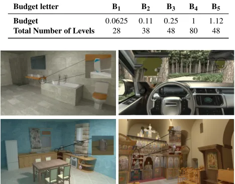
Table 2. Theoretical budgets used in this experimental study along with their notation letters and the number of quality levels available when a budget is applied.

Budget letter B1 B2 B3 B4 B5

Budget 0.0625 0.11 0.25 1 1.12

Total Number of Levels 28 38 48 80 48

Fig. 5. Scenarios of this experimental study. From Left to Right and Top to Bottom: Bathroom, Car, Kitchen, Kitti. The circular areas show the smell source.

The wide range of budget sizes (B1-B5) allows to investigate users’

allocation preferences both with and without budget constraints. Using

equation 7, andM=1K, the normalized costs for the smell impulse

can be computed for all four scenarios of interest. The theoretical cost for smell was estimated using the physical computation times obtained

from the coarsest mesh size, therefore, the selection of 1Kis justified

from the findings of Experiment I, where the selection of the mesh size for simulating smell transport has no perceptual effect to the user.

Table 3. Theoretical costs for smell across the four scenarios selected. The first row shows the virtual time (sec) required to reach concentration C1. The second row shows physical computation times (sec) for the

coarsest mesh (1K). The third row shows physical computation times (sec) for the finest mesh (1M). The last row gives theoretical costs for smell as ratios of the second and third row.

Scenario

Bathroom

Car

Kitchen

Kitti

V T

646

458

1685

1199

PT

229

.

2

123

.

6

718

.

8

481

.

3

PT

6222

.

5

4164

.

7

17900

.

3

15228

.

9

A

0

.

037

0

.

029

0

.

040

0

.

032

5.2 Materials

For this study, two monitors (First: 2800Samsung U28D590 ultra HD

LED monitor used for visual stimuli, Second: Dell UltraSharp 1900used

for the GUI) and a set of headphones (Sennheiser HD 380 pro) were used for conducting this experiment. In addition, the olfactory display used of the preliminary experimental study was used for the delivery of the smell impulses. All the experimental trials were conducted in a silent room with constant ventilation. The same four scenarios used for smell transport simulations in Experiment I were used. The smell of citral, was congruent to all of them. Figure 5 depicts the experimental scenarios and zooms in the source of smell used for the simulation of odour transport. From the user’s perspective, at least one object could have been the source of smell and no information was given to the participants regarding the source of the odour. A GUI application was used for carrying out the experimental study, see Figure 6.

Fig. 6. Snapshots of the software used in the experimental study. Left: An instance of the budget sizeB2when the “Smell OFF” control is activated.

Right: An instance of the budget sizeB2when the “Smell ON” control is

activated.

for audio-visual quality improvements are reduced. When the control for smell was turned on, a smell impulse of 1 second was delivered to the user at close vicinity to the nose. The delivery of smell bursts instead of a continuous flow was preferred so as to avoid user’s fast adaptation to the released odour. A control channel was also used to

release air bursts of 1,000 ml/min flow rate and convect the smell bursts

away from participant’s location. Five air burst of frequency 400 ms were released when the user was pressing the “Next” or the “Smell OFF” buttons to go to the next trial or choose not to allocate resources when the “Smell ON” was enabled respectively. The delivery of the audio and visual stimuli was delayed by 240 ms when the smell was set on in the experiment to compensate the olfactory display’s onset time. The objective was to deliver all three sensory stimuli simultaneously without the participants perceiving temporal delays.

The use of the air channel was very important as it didn’t allow adaptation of the user to the smell cue. The air channel intended to disperse the smell plume quickly at the ventilation system which was right behind and above participant’s head. Also in situations where participants wanted to try the smell cue and disable it immediately, the air channel assisted to remove the residues of the smell out immediately in an attempt to disable the sensory cue as quickly as possible.

At the beginning of each experimental trial the two sliders are po-sitioned at the start of the slider bars which correspond to a “null” stimulus. The “null” stimulus configuration includes the delivery of a grey image and a silent track while the smell control is pre-selected to be “OFF”. The initial selection of the grey image aims to neutralize

par-ticipants’ eyes and is suggested by [1]. When budgetB5is available for

resource allocation, the audio and visual thumbs start from a medium

quality level that has cost equal toB5−B4. The initial configuration of

the thumbs allows the participants to explore all the available quality levels before deciding which quality level is desired. The alternative option to start the thumbs at random positions was not preferred to avoid biasing the participant with a thumb configuration which does not represent his/her actual preferences. At the beginning of each trial, the two thumbs are independent of each other until the sum of the theoretical costs for the three sensory stimuli exceeds the budget given for the trial. After the first attempt to exceed the budget, the thumb controls become dependent. At any point, if the user activates the smell impulse, the GUI sliders adjust to the new lower budget.

The transition from independent to dependent slider controls for adjusting audio-visual quality changes to either the senses of vision or hearing the quality of the other stimulus so as the budget to remain always constant and equal to the current budget size. The addition of the olfactory impulses does not disrupt this mechanism as the cost for a smell impulse is immediately allocated after the control is turned on.

5.3 Participants and Procedure

A total of 25 participants (13m, 12f, age range: 23 to 46,µ=36.2)

volunteered. All of them had normal or corrected to normal vision. None of them reported hearing or temporary/permanent smell problems. All the participants recruited for this experiment had no participation in Experiment I or were aware of its purpose.

Every experimental session was initiated with a tutorial where the

participants had the chance to familiarize with the task of allocating resources. The Kitti scenario was used for training with all possible budgets. During the tutorial, the experimenter had the chance to explain the objectives and purpose of the study to the participants for about 15 minutes before the main session. The participants were asked to judge and form the best multi-sensory experience using the controls of the GUI.

5.4 Results

The analysis of the results is divided into two parts for better clarity.

The first part includes an ANOVA via a 3 (scenario)× 5 (budget)

factorial design for studying the effect of the independent variables on participants’ decision to enable the smell impulse on and the second part describes a multivariate analysis of variance (MANOVA) for examining the effect of the two independent variables on the visual and auditory allocation preferences.

5.4.1 Analysis of the smell preferences

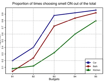
Figure 7 depicts the proportion of times that people preferred to receive a smell impulse along with an audio/visual stimulus for each of the three scenarios and across every budget. At small budget sizes, participants choose not to allocate resources for enabilng the olfactory stimuli. As the budget increases, the frequency people select to receive an olfactory stimulus increases significantly. Furthermore, people tend to enable the control for smell more often in the Car and Bathroom VEs compared to the Kitchen VE. Participants’ preference to these scenarios might be explained due to the ease of visually locating the smell source in the scene.

B1 B2 B3 B4 B5

0.1

0.2

0.3

0.4

0.5

0.6

0.7

0.8

0.9

Budgets

Proportion

Proportion of times choosing smell ON out of the total

Car Bath Kitchen

Fig. 7. Proportion of times smell stimulus was set on in each of the three scenarios and across all different budgets.

The main effect of budget was significant withF(4,96) =61.47,

p<0.05 indicating a difference in the proportions the subjects selected

to receive a smell impulse across the five budgets. The main effect of budget did not violate the assumption of sphericity (via Maulchy’s test,

p>0.05). The main effect of scenario was also significantF(2,48) =

18.42,p<0.05 indicating a difference in the proportions the smell

burst was received by the participants across the three scenarios. The main effect for scenario did not also violate the assumption of sphericity.

The interaction of budget×scenario was also examined and it was not

found to be statistically significant,F(8,192) =1.76,p>0.05.

Contrast comparisons for proportions were conducted between groups of budgets using post-hoc proportion tests with Bonferroni corrections. These results are presented in Table 4. The results show

that small budget sizes (B1,B2) are not significantly different indicating

that the budget size is still not sufficient for distributing resources to

smell. Large budget sizes are also not significantly different (B4,B5)

meaning that people tend to enable the smell stimulus approximately the same number of times during their allocation.

Contrast comparisons for proportions were also conducted between groups of scenarios using post-hoc proportion tests and applying

Scenario Budget size p−value

Car B1 B2 B3 B4 B5 <0.05

Bath B1 B2 B3 B4 B5 <0.05

Kitchen B1 B2 B3 B4 B5 <0.05

All B1 B2 B3 B4 B5 <0.05

Table 4. Contrast comparisons for proportions of smell between bud-gets. Proportions of budgets with no significant differences are grouped together.

For the remaining three budget sizes, the group{Car, Bath}is

signifi-cantly different from the group{Kitchen}indicating that participants

clearly prefer to enable the smell on more frequently at scenarios of the former group.

5.4.2 Analysis on the audio-visual preferences

Figure 8 depicts the mean percentages and confidence intervals for graphics and acoustics quality for each scenario and budget. As can be seen, the visual and auditory percentages are negatively correlated. For small budget sizes participants prioritise visuals and allocate the major-ity of the budget. As the budget size increases a balanced distribution of resources is preferred as the available amount permits it.

0 10 20 30 40 50 60 70 80 90 100

B1 B2 B3 B4 B5

Budgets

Graphics allocation (%)

Scenario Car Bath Kitchen

Means and confidence intervals for Graphics

0 10 20 30 40 50 60 70 80 90 100

B1 B2 B3 B4 B5

Budget

Acoustics allocation (%)

Scenario Car Bath Kitchen

Means and confidence intervals for Acoustics

Fig. 8. Mean allocation percentages and confidence intervals for every scenario and across all the budget sizes Top: Graphics, Bottom: Acous-tics. Jittering has been applied to the two plots for better visualisation.

MANOVA analysis was applied to examine the effect of the bud-get and scenario on the audio-visual allocation percentages. For the acoustic quality percentage, the main effect of budget was significant

withF(4,96) =153.85,p<0.05 while the effect of scenario was not

found to be statistically significant withF(2,48) =0.0241,p>0.05.

The main effect of budget and scenario did not violate the assumption

of sphericity (via Maulchy’s test,p>0.05). The interaction scenario

×budget was not found significant,F(8,196) =0.012p>0.05.

For the visual quality percentage, the main effect of budget was

significant withF(4,96) =42.11, p<0.05. The effect of scenario

was also found to be statistically significant for the graphics allocation

percentage withF(2,48) =11.03,p<0.05. The main effect of both

factors did not violate the assumption of sphericity (via Maulchy’s test,

p>0.05). The interaction scenario×budget was not found significant,

F(8,196) =0.94,p>0.05.

Contrast comparisons using post-hoc t-tests were also conducted to investigate groups of budgets that are not significantly different across the scenarios and also for finding groups of scenarios that are not significantly different across budgets. These contrasts are given in Table 5 and Table 6 for graphics and acoustics respectively.

Scenario Budget size p−value

Car B1 B2 B3 B4 B5 <0.05

Bath B1 B2 B3 B4 B5 <0.05

Kitchen B1 B2 B3 B4 B5 <0.05

All B1 B2 B3 B4 B5 <0.05

Budget Scenarios p−value

B1 Car Bath Kitchen <0.05

B₂ Car Bath Kitchen <0.05

B₃ Car Bath Kitchen <0.05

B₄ Car Bath Kitchen <0.05

B₅ Car Bath Kitchen <0.05

All Car Bath Kitchen <0.05

Table 5. Left: Contrast comparisons between budgets at every scenario and across all the scenarios for graphics. Right: Contrast comparisons between scenarios at every budget and across all the budgets for graph-ics. Budgets or scenarios with no significant difference are grouped together.

As can be seen from Table 5, small budget sizes (B1,B2) are not

sig-nificantly different meaning that participants follow similar allocation strategy for graphics for these budgets independently of the scenario.

The same argument also holds for very large budget sizes (B4,B5). As

far as the scenarios are concerned, subjects tend to increase graphics quality in a similar way for the Kitchen and Bath scenarios.

Scenario Budget size p−value

Car B1 B2 B3 B4 B5 <0.05

Bath B1 B2 B3 B4 B5 <0.05

Kitchen B1 B2 B3 B4 B5 <0.05

All B1 B2 B3 B4 B5 <0.05

Budget Scenarios p−value

B1 Car Kitchen Bath <0.05

B₂ Car Kitchen Bath <0.05

B₃ Car Kitchen Bath <0.05

B4 Car Kitchen Bath <0.05

B₅ Car Kitchen Bath <0.05

All Car Kitchen Bath <0.05

Table 6. Left: Contrast comparisons between budgets at every scenario and across all the scenarios for acoustics, Right: Contrast comparisons between scenarios at every budget and across all the budgets for acous-tics. Budgets or scenarios with no significant difference are grouped together.

Table 6 shows that none of the scenarios is significantly different from the others when distributing resources for aural quality improve-ments. As far as the budgets are concerned, the same trend for graphics holds also for the acoustics for the effect of the budget size.

6 ESTIMATION MODEL

The experimental data was used in the construction of a statistical model which aims to estimate three quantities given a budget, and optionally the scenario. The first quantity is the probability that expresses whether smell should be given for an input budget and scenario while the other two estimations are proportions of the total budget that should be devoted to visual and aural quality.

As the decision to turn the smell stimulus on or off is based on a categorical variable, a logistic regression was used to model it.

Specif-ically, if the probability to give a smell impulse is denoted aspthen

the ratio ₁₋p_pexpresses the odds of enabling the smell impulse release.

This smell on/off decision can be modeled as:

log p

1−p

=βˆ_is+βˆ_bs·budget+1S·γˆ_Ss, (8)

where the coefficients ˆβ_is, ˆβ_bsand ˆγ_Ssare the least squares regression

estimates. The subscriptsiandbare shorthand for the intercept and

the budget respectively, and the subscriptSis shorthand for scenario.

The motivation for scenario specificity is dictated by the significant differences identified between the scenarios in the experimental data.

ˆ

the model for each scenario. The indicator function1Sdenotes whether

the scenario is included as part of the model.

For an input budget size, if the signum of the right hand side of

Equation 8 is positive then it can be inferred thatp>1−pand thus a

smell impulse should be delivered to the user. The above model is used to estimate whether the smell should be turned on/off and is only one component of the whole model. The full model is also composed of audio-visual percentage allocation components and can be written in matrix form as:





ˆ

S1

ˆ

V1

ˆ

A1



= 



ˆ

β_is βˆ_bs γˆ_Ss

ˆ

β_iv βˆ_bv γˆ_Sv

ˆ

β_ia βˆ_ba γˆ_Sa 

· 



1 budget

1S



, (9)

where the letters ˆV1and ˆA1are the vision and audio allocation

estima-tions while ˆS1=log

_p

1−p

is the model component for smell as given in formula 8.

The remainder of the paper will consider two forms of the model for

both testing and evaluation:M1refers to1S=0 where the scenario is

not considered, andM2refers to1S=1 which considers the scenario

in the model.

ForM1, hypothesis tests of the form:

H0:βzk=0 vsHa:βzk6=0, z∈ {i,b}andk∈ {s,v,a}

were conducted to check the significance of the unknown

parame-tersβis,βbs,β

v i,β

v b,β

a

i,βba. In all these tests the null hypothesis is

re-jected indicating that the respective least squares regression estimators

( ˆβ_is,βˆ_bs,βˆ_iv,βˆ_bv,βˆ_ia,βˆ_ba) should remain in the model formulation. The

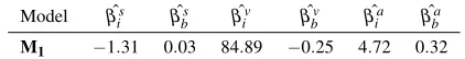
six estimates on the right hand side of the above equation are given in Table 7.

Model βˆ_is βˆ_bs βˆ_iv βˆ_bv βˆ_ia βˆ_ba

M1 −1.31 0.03 84.89 −0.25 4.72 0.32

Table 7. Least squares regression estimates of the multivariate model

M1. The subscripts “i” and “b” are used as shorthands for intercept and

budget respectively. The superscipts “s”, “v”, “a”, are used instead of smell, vision and audio respectively.

The coefficients of determinationR2andR2_adjfor the goodness of fit

for modelM1are given in Table 8. The superscript in parenthesis is

used to denote the sense. As the smell estimation is based on logistic regression the first coefficient of determination is based on the Akaike Information Criterion (AIC) (the lower the better) while the other two for graphics and audio are the Nagelkerke coefficients of determination (the higher the better).

Model R2(s) R2(v) R_adj2(v) R2(a) R2_adj(a)

M1 24.80 0.37 0.36 0.61 0.61

M2 18.40 0.40 0.40 0.65 0.62

Table 8. Coefficients of determination for the multivariate modelsM1

andM2. The Akaike information criterion was used for theR2(s). The

Nagelkerke coefficient is used for vision and audio.

M2considers the scenario as input to the model, and therefore can

better match the experimental results thanM1which is based an the

average across all scenarios.M2introduces extra parametersγ_Ss,γ_Svand

γ_Sawhich are examined to see whether they are statistically significant

and should be kept in the modelM2. Hypothesis tests of the following

form:

H0:γ_Sk=0 vsHa:γ_Sk6=0, k∈ {s,v,a}, (10) were conducted to see the significance of these parameters in the

Kitchen and Car scenario. For the Kitchen scenario (S=K), it was

found that for the parameterγ_KvtheH0is not rejected (p>0.05) and the

same also holds for the parameterγ_Ka. For the car scenario,γ_Cais also

not rejected. The latter parameters were expected to be not significant

as the factorscenariowas not found to be statistically significant for

adjusting aural quality in the MANOVA tests of the previous section. All the other parameters were found statistically significant (reject the

H0).

The least square regression estimates of theM2model are given

in Table 9, and the coefficients of determinationR2andR2_adjfor the

goodness of fit for modelM2are given in Table 8.

Sense βˆi βˆb γˆC(Car) γˆK(Kitchen)

Smell −1.35 0.04 0.72 −1.10

Visual 87.33 −0.25 −7.29 ∗

Audio 4.72 0.32 ∗ ∗

Table 9. Least squares regression estimates of the multivariate modelM2.

The asterisks show the parameters that are not statistically significant (not reject theH0hypothesis) and their estimators were excluded from

the statistical model.

7 EXPERIMENTIII: MODELVALIDATION

The performance of the model was validated in an experimental study which included the use of untested budget sizes and a new untested scenario to test the performance of the model with inputs other than the ones used for the construction.

7.1 Design

The validation study follows the same guidelines as the main experi-mental study. Three scenarios were used, namely, Car, Kitchen and Kitti. Kitti was the new scenario for the validation stage (this was only used for training previously). Three budgets were used in this experi-ment, each one different from the previously used budgets. These were

the midpoints betweenB1andB2,B2andB3andB3andB4. These

are denoted asNB1,NB2andNB3. All the materials of the main study,

were also used for the validation stage with no change. The Kitchen scenario was used for training. A total of six people participated and none of these participants were familiar with the objectives of the ex-periment as they had not taken part in the previous exex-periments. We

test bothM1andM2, and for the scenario specific coefficients forM2

we used the values from the Car scenario based on the rationale that the smell source has a similar configuration to the Car scenario.

7.2 Results

M1andM2were compared with the data collected from the validation

study to investigate their performance against real human preferences. Figure 9 shows the means and confidence intervals for results for all scenarios and modalities. The model estimations are also depicted as colored curves for comparison. For graphics, the average error for

absolute difference for theM1 is 5.8% while forM2 is 2.3%. For

acoustics,M1andM2give an average error of absolute difference of

3.4%. For small budgets (NB1) bothM1andM2predict equally well

for graphics quality. As the budget size increases, modelM2gives

more accurate estimations.

For the Kitchen scene, for graphics, the average error for absolute

difference is 4.4% and 1.6% forM1andM2respectively. For acoustics,

M1andM2give an average error of absolute difference of 2.3%. For

smell, at small budget sizes people prefer a low quality audio while

smell is not set on. For the test budgetsNB1andNB2,M1andM2

overestimate for audio and smell while they underestimate for graphics.

For the new Kitti scenario, whose data wasnotused to buildM1

orM2, for graphics the average error for absolute difference is 1.6%

and 5.8% forM1 andM2 respectively while for acousticsM1 and

M2give an average error of absolute difference of 4.9% indicating

that participants’ need for acoustic quality was significantly increased

NB1 NB2 NB3 56 60 64 68 72 76 80 84 88 Budgets

Graphics allocation (%)

Models validation for Graphics-Car

M1 M2(C)

NB1 NB2 NB3

0 4 8 12 16 20 24 28 32 36 40 44 48 Budgets

Acoustics allocation (%)

Models validation for Acoustics-Car

M1-M2

NB1 NB2 NB3

0.0 0.1 0.2 0.3 0.4 0.5 0.6 0.7 0.8 0.9 1.0 Budgets

Probability of smell ON

Models validation for Smell-Car

M1

M2(C)

NB1 NB2 NB3

56 60 64 68 72 76 80 84 88 Budgets

Graphics allocation (%)

Models validation for Graphics-Kitchen

M1

M2(K)

NB1 NB2 NB3

0 4 8 12 16 20 24 28 32 36 40 44 48 Budgets

Acoustics allocation (%)

Models validation for Acoustics-Kitchen

M1-M2

NB1 NB2 NB3

0.0 0.1 0.2 0.3 0.4 0.5 0.6 0.7 0.8 0.9 1.0 Budgets

Probability of smell ON

Models validation for Smell-Kitchen

M1

M2(K)

NB1 NB2 NB3

56 60 64 68 72 76 80 84 88 Budgets

Graphics allocation (%)

Models validation for Graphics-Kitti

M1

M2(C)

NB1 NB2 NB3

0 4 8 12 16 20 24 28 32 36 40 44 48 Budgets

Acoustics allocation (%)

Models validation for Acoustics-Kitti

M1-M2

NB1 NB2 NB3

0.0 0.1 0.2 0.3 0.4 0.5 0.6 0.7 0.8 0.9 1.0 Budgets

Probability of smell ON

Models validation for Smell-Kitti

M1 M2(C)

Fig. 9. Left and Middle: Means and confidence intervals for the three scenarios for graphics and acoustics respectively. The green curve showsM1

and the red showsM2. The (K) or (C) notations ofM2denote coefficients from the Kitchen or Car scenario as used inM2. Log-spacing was applied

to thex-axis for better visualisation. Right: Proportion of times smell was preferred on for each of the test budgets across the three scenarios. The green and red curves are the probability estimations to turn the smell on forM1andM2respectively.

8 DISCUSSION

The results yield a number of potentially useful findings related to the way humans tend to allocate resources in tri-modal VEs. The co-existence of more than two senses in the experimental set-up does not affect humans’ general trend to devote the majority of their budget for visual quality improvements. For the scenarios used and the smaller budget sizes, people’s priority is to obtain a clear visual stimulus while compromises are made to both the audio quality and the addition of smell. As more resources become available, participants prefer an approximately balanced distribution of resources while the frequency with which smell was added was significantly increased.

As far as the effect of the scenario is concerned, it is clear that the four scenarios affect people’s decision to enable the release of smell impulses. The scenario selection was also important for the visual allocation preferences while it had no effect on the percentage devoted to aural quality improvements. Participants did not show significant differences in acoustic resource allocation across the scenarios.

The validation stage shows evidence that the statistical model pro-vides allocation estimates of different accuracy, especially in the case

of the visual percentages.M1, the generic version of the model, gives

relatively accurate predictions but it was outperformed by modelM2

in almost all the combinations of budget-scenario test conditions. The

results of the validation study indicate also that bothM1andM2give

relatively accurate estimations for the three different validation budgets

and scenario. When usingM2, results are improved at the cost of scene

dependent parameters, which currently require experiments to deter-mine. This is an area of future work, as it is likely that these parameters can be predicted as a function of the multi-modal content of the scene. The delivery of the visual stimuli as static images is a limitation of this experimental study as it restricts the number of possible ap-plications of the proposed estimation model. Both the auditory and

olfactory stimuli have an inherent temporal dimension (duration of the audio track/smell burst) that is not exploited with the use of static visual images. However, the experimental methodology can provide useful insights on extending to VEs with animations or interactive environments.

Another possible limitation is the use of the binary (on/off) smell stimuli. It can be said that the two-level methodology for deliver-ing smell impulses restricts user’s available options but it is not clear whether (and how) a hypothetical multiple quality scale for smell would benefit user’s virtual experience, particularly with current olfactory hardware limitations, as shown in Experiment I. The existence of mul-tiple smells, on the other hand, is considered more important in a multi-sensory VE and can admittedly increase the level of immersion as it is closer to what happens in the real word. To that end, the JND estimation methodology can be applied in arbitrary number of VOCs or combinations of them.

9 CONCLUSION