warwick.ac.uk/lib-publications
A Thesis Submitted for the Degree of PhD at the University of Warwick
Permanent WRAP URL:
http://wrap.warwick.ac.uk/117383
Copyright and reuse:
This thesis is made available online and is protected by original copyright. Please scroll down to view the document itself.
Please refer to the repository record for this item for information to help you to cite it. Our policy information is available from the repository home page.
Radiative Heat Transfer for Modelling Fire and Fire Suppression
Submitted to the University of Warwick
1
Radiative Heat Transfer for Modelling Fire and Fire Suppression
by
Ivan Sikic
Thesis
Submitted to the University of Warwick
for the degree of
Doctor of Philosophy
School of Engineering
March 2018
2
Table of contents
List of Figures ... 7
List of Tables ... 12
Acknowledgements ... 14
Declarations ... 15
Abstract ... 16
Nomenclature ... 17
Chapter 1 - Introduction ... 21
1.1. Radiative properties of non-grey gases in fires ... 21
1.2. Radiative properties of particulates in fires or fire suppression ... 24
1.3. Motivation, aims & objectives and contributions of the thesis ... 24
1.4. Layout of the thesis ... 25
Chapter 2 - Literature review ... 27
2.1. Overview of solution methods for the radiative transfer equation (RTE) ... 27
2.2. The weighted-sum-of-grey-gases (WSGG) model... 28
2.3. Exponential wide band (EWB) and box models ... 29
2.4. WSGG and EWB/box models in CFD codes and fire simulations ... 29
2.5. Fire suppression by water sprays ... 31
Chapter 3 - Mathematical modelling ... 33
3.1. Governing equations ... 33
3.2. The general radiative transfer equation ... 34
3.2.1. Blackbody intensity... 34
3.2.2. Radiative heat flux ... 34
3
3.2.4. Scattering... 35
3.2.5. Energy conservation ... 36
3.3. Non-scattering media ... 36
3.4. Solutions of the non-scattering RTE ... 37
3.5. Mean beam lengths ... 38
3.6. Angular and spatial discretisation of the non-scattering RTE ... 39
3.7. Weighted-sum-of-grey-gases (general formulation) ... 40
3.7.1. Grey WSGG ... 41
3.7.2. Banded or non-grey WSGG ... 41
3.8. The three sets of WSGG correlations implemented in FireFOAM ... 42
3.9. Exponential wide band (EWB) and "box" models ... 45
3.9.1. Exponential wide band (EWB) ... 46
3.9.2. Box model ... 49
3.9.3. Band overlaps ... 51
3.9.4. Relevant simplifications for computational efficiency ... 53
3.9.5. Parameter scaling for inhomogeneous path lengths ... 54
3.10. Radiative properties of soot ... 55
3.11. Combustion, soot and turbulence models in FireFOAM ... 56
3.12. Summary ... 57
Chapter 4 - Results and discussion (pure radiation cases) ... 58
4.1. Investigation of the weighted-sum-of-grey-gases (WSGG) in static media (pure radiation only cases) ... 59
4.1.1. Grey gas in a 2D enclosure ... 60
4.1.2. Hot surface emitting through transparent gas in a 3D cylinder ... 61
4.1.2.1. Wide emitting surface ... 61
4.1.2.2. Smaller emitting surface ... 64
4
4.1.3.1. One-dimensional gas mixture with soot loadings ... 66
4.1.3.2. Non-isothermal mixture in 2D enclosure ... 67
4.1.3.3. Pure H2O in 3D enclosure ... 69
4.1.4. Inhomogeneous gases ... 71
4.1.4.1. One-dimensional gas mixture with soot loadings ... 71
4.1.4.2. Pure CO2 or pure H2O in 2D enclosure ... 74
4.1.4.3. Pure H2O in 3D enclosure ... 77
4.1.5. Summary ... 80
4.2. The exponential wide band box model ... 80
4.2.1. Introduction ... 80
4.2.2. Variable band models in static media ... 80
4.2.2.1. Non-overlapping bands, single gas species, homogeneous media ... 80
4.2.2.1.1. 2D pure CO2 ... 81
4.2.2.1.2. 2D pure H2O ... 83
4.2.2.1.3. 3D pure H2O ... 85
4.2.2.2. Non-overlapping bands, single gas specie, inhomogeneous media ... 87
4.2.2.2.1. 2D pure CO2 ... 88
4.2.2.2.2. 2D pure H2O ... 90
4.2.2.2.3. 3D pure H2O ... 91
4.2.2.3. Overlapping bands, mixtures of two absorbing gas species ... 93
4.2.2.3.1. 1D homogeneous gas mixture ... 94
4.2.3. Bandwidth sensitivity study with the variable band box models ... 98
4.2.4. Estimation of mass path length range for pool fires ... 102
4.2.5. Estimation of band strengths (full emissivity data) ... 106
4.2.6. Modest-based fixed bands box model in static media ... 109
4.2.6.1. Homogeneous media... 111
5
4.2.6.1.2. 2D pure H2O ... 112
4.2.6.1.3. 3D pure H2O ... 114
4.2.6.1.4. 1D mixture ... 116
4.2.6.2. Inhomogeneous media ... 118
4.2.6.2.1. 2D pure CO2 ... 118
4.2.6.2.2. 2D pure H2O ... 119
4.2.6.2.3. 3D pure H2O ... 121
4.2.6.2.4. 2D non-isothermal mixture ... 122
4.2.7. Box model for pool fires ... 125
4.2.7.1. Flame volume-based scaling method ... 125
4.2.7.2. Spectral modelling of 30cm methanol and heptane fires with the box models ... 130
4.2.8. Summary ... 131
Chapter 5 - Results and discussion (pool fire cases) ... 133
5.1. Introduction and objectives ... 133
5.2. Simulation parameters and CPU times ... 135
5.3. Large eddy simulations of 30cm methanol fires ... 136
5.3.1. Grid independence and effect on temperature prediction ... 136
5.3.2. Influence of TRI parameters ... 137
5.3.3. Comparison of gas radiation approaches ... 140
5.4. Large eddy simulations of 30cm heptane fires ... 142
5.4.1. Grid independence and effect on temperature and soot predictions ... 142
5.4.2. TRI parameters, radiant fluxes ... 145
5.5. Large eddy simulations of 60cm pool fires ... 146
5.5.1. Temperatures ... 148
5.5.2. Radiative fluxes and fractions ... 148
6
Chapter 6 - Results and discussion (two-phase flows) ... 153
6.1. Basic aspects of Mie theory... 153
6.2. Overview of the original implementation ... 155
6.3. Adaptation for coupling with gas phase box model ... 156
6.4. Preliminary test cases ... 158
6.4.1. Liquid phase only, 1D slab ... 158
6.4.2. Coupled radiation of liquid and gas phases in a 3D enclosure ... 159
6.5. Summary ... 161
Chapter 7 - General conclusions, recommendations and further
studies ... 162
7
List of Figures
1-1 Large scale hydrocarbon pool fire (internet at large) ... 22
1-2 Small portion of the absorption-emission spectrum of water vapour (NIST)... 22
1-3 Narrow band modelling of the 4.3µm rotation-vibrational region of CO2 ... 23
1-4 Wide band modelling of the 71µm (140cm-1) rotational region of H2O ... 23
3-1 Optical path between two arbitrary points in an arbitrary medium ... 35
3-2 Radiative scattering from unit volume dV ... 36
3-3 Isothermal gas volume radiating to surface element for (a) an arbitrary gas volume, and (b) for an equivalent hemisphere radiating to the centre of its base where Le = mean beam length ... 38
3-4 Band shapes with the exponential wide band model (left: upper band head, centre: symmetric band head, right: lower band head) ... 46
3-5 Band shape with the box model ... 46
3-6 Plots of the Planck fractional energy function, calculated with Eq. 3.75 for different temperatures ... 51
3-7 "Beer" box model absorption spectrum for 35% H2O, 65% CO2, path length 9.4m, T=1500K ... 52
3-8 Turbulent energy cascade in the LES framework (reproduced from [23]) ... 56
4-1 Sketch of 2D and 3D geometries employed in [35] and [34] respectively ... 59
4-1-1 Radiative source term along (x, y = 0.25) and (x = 0.5, y) (top), incident flux along (x, y = 0.5) and (x = 1, y) (bottom) for the 2D grey gas case of [35], FireFOAM-FVM vs RTM of [35] ... 60
4-1-2 View of the transparent cylinder mesh and temperature field (a), locations of the radiative flux line plots (b) (z = 10cm, 1m, 1.90m) ... 62
4-1-3 Evolution of the incident radiative flux along the cylinder circumference, at height z = 1m above the emitting region (modified case with Remission = 15cm). Showing dependence on discretisation of azimuthal angle φ ... 64
4-1-4 Evolution of the incident radiative flux vertically along the cylinder's side wall at R = 1m for the modified emission surface case. Showing dependence on discretisation of polar angle θ ... 65
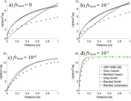
4-1-5 Comparison of FireFOAM-WSGG line-of-sight solutions with DBT-SNB from [36] for different soot volume fractions (isothermal & homogeneous gas) ... 66
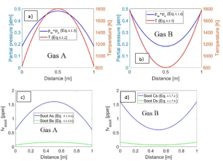
4-1-6 Temperature field from Eq. 4.1.1 in 1m x 0.5m enclosure of [35] ... 67
4-1-7 (a), (b) Radiative source term along (x, y = 0.25) and (x = 0.5, y), (c), (d) incident flux along (x, y = 0.5) and (x = 1, y) for the non-isothermal 2D enclosure of [35], FireFOAM-WSGG vs SNB of [35]... 69
4-1-8 (a), (b) Radiative source term along (x = 1m, y = 1m, z) and (x, y = 1, z = 0.375m) ; (c), (d) incident flux along (x = 2m, y = 1m, z) and (x, y = 1m, z = 4m) for the 3D enclosure of [34], FireFOAM-WSGG vs SNB of [34,84] ... 70
4-1-9 Errors of FireFOAM-WSGG relative to SNB [34,84], on the radiant source term (a, b) and flux (c, d) from Fig. 4-1-8 ... 70
8
4-1-11 Comparison of FireFOAM-WSGG line-of-sight solutions with DBT-SNB from [36] for different soot volume loadings (non-isothermal, inhomogeneous) ... 73 4-1-12 Temperature field from Eq. 4.1.8 in 1m x 0.5m enclosure of [35] ... 74 4-1-13 FireFOAM-WSGG vs SNB of [35] in 2D inhomogeneous and non-isothermal CO2 case of [35], (a), (b) radiative source term along (x, y = 0.25) and (x = 0.5, y), (c), (d) incident flux along (x, y = 0.5) and (x = 1, y) ... 75 4-1-14 Errors of FireFOAM-WSGG relative to SNB [35], on the radiant source term (a, b) and flux (c, d) from Fig. 4-1-13 ... 76 4-1-15 FireFOAM-WSGG vs SNB of [35] in 2D inhomogeneous and non-isothermal H2O case of [35], (a), (b) radiative source term along (x, y = 0.25) and (x = 0.5, y), (c), (d) incident flux along (x, y = 0.5) and (x = 1, y) ... 76 4-1-16 Errors of FireFOAM-WSGG relative to SNB [35], on the radiant source term (a, b) and flux (c, d) from Fig. 4-1-15 ... 77 4-1-17 (a), (b) Radiative source term along (x = 1m, y = 1m, z) and (x, y = 1, z = 0.24m) ; (c), (d) incident flux along (x = 2m, y = 1m, z) and (x, y = 1m, z = 4m) for the
inhomogeneous 3D gas of [34], FireFOAM-WSGG vs SNB of [34,84] ... 78 4-1-18 Errors of FireFOAM-WSGG relative to SNB [34,84], on the radiant source term (a, b) and flux (c, d) from Fig. 4-1-17 ... 79 4-2-1 Absorption spectrum of CO2 at X = 35.93 g/m2 ... 81 4-2-2 Comparison of box models vs SNB of [35], source term along x and y (top), heat flux along x and y (bottom) for CO2 at X = 35.93 g/m2 ... 82 4-2-3 Box model absorption spectra of H2O at X = 29.39 g/m2, with (left) and without (right) the pure rotational 140 cm-1 band ... 83 4-2-4 Source term along x and y (top), heat flux along x and y (bottom) for pure H2O with X = 35.93 g/m2, with and without the 140 cm-1 band ... 84 4-2-5 Box model absorption spectra of H2O at X = 316 g/m2 ... 85 4-2-6 Comparison of box models vs SNB of [34,84], source term along x and z (top), heat flux along x and z (bottom) for pure H2O with X = 316 g/m2 ... 86 4-2-7 For the inhomogeneous CO2 and H2O cases from Goutiere et al. [35], (a)
9
4-2-15 Box model absorption spectra of CO2-H2O mixture with XCO2 = 65.6 g/m2 and
XH2O = 80.1 g/m2... 94 4-2-16 Line of sight intensity of each band from Modest (left) and Beer (right) models, for CO2-H2O mixture with XCO2 = 65.6 g/m2 and XH2O = 80.1 g/m2 ... 95 4-2-17 Line of sight total intensities for CO2-H2O mixture with XCO2 = 65.6 g/m2 and
XH2O = 80.1 g/m2... 96 4-2-18 Evolution of line-of-sight radiant intensity in CO2-H2O mixture with XCO2 = 65.6 g/m2 and XH2O = 80.1 g/m2 ... 97 4-2-19 to 4-2-40 Box model bandwidth as a function of pressure-path length for
different temperature, comparing Modest and Beer models in each CO2 and H2O band ... 98-102 4-2-41 Centreline distributions of pressure path length (blue) and mass path length (red) in four pool fires of different fuels, heat release rates and diameters ... 103 4-2-42 Comparing different methods for mean beam length calculations in pool fires, i.e. the integral length scale (solid line), the cylindrical approximation ('x' symbols) and the conical approximation ('o' symbols) ... 104 4-2-43 to 4-2-53 Box model band emissivities as a function of pressure-path length for different temperatures... 107-108 4-2-54 Box model absorption spectra of pure CO2 with X = 35.9 g/m2 ... 111 4-2-55 Box model vs. SNB from [35], source term along x and y (top), heat flux along x and y (bottom) for CO2 at X = 35.93 g/m2 ... 112 4-2-56 Absorption spectrum of pure H2O with X = 29.4 g/m2, with (left) and without (right) the pure rotational band 140cm-1... 113 4-2-57 Box model vs SNB from [35], source term along x and y (top), heat flux along x and y (bottom) for H2O at X = 29.4 g/m2 ... 114 4-2-58 Absorption spectrum of pure H2O with X = 316 g/m2 ... 115 4-2-59 Box model vs. SNB from [34], source term along x and z (top), heat flux along x and z (bottom) for pure H2O with X = 316 g/m2 ... 116 4-2-60 Box model absorption spectra of CO2-H2O mixture with XCO2 = 65.6 g/m2 and
XH2O = 80.1 g/m2, with (left) and without (right) rotational band at 140cm-1 ... 117 4-2-61 Line of sight total intensities for CO2-H2O mixture with XCO2 = 65.6 g/m2 and
10
4-2-68 Box model absorption spectra of nonisothermal mixture with XCO2,ave = 37 g/m2and XH2O,ave = 30g/m2, with fixed bands model (left) and variable band models (right) ... 123 4-2-69 Box model vs SNB from [35], source term along x and z (top), heat flux along x and z (bottom) for nonisothermal mixture with XCO2,ave = 37 g/m2 and XH2O,ave = 30g/m2 ... 125 4-2-70 Left to right, transient temperature, CO2 and H2O mass fractions, absorption coefficient from scaled parameters and flame volume based on temperature elevation method ... 126 4-2-71 Box model absorption spectra of 20kW methanol flame, scaled at 40% of the total volume ... 127 4-2-72 Box model absorption spectra of 20kW methanol flame, scaled at 30% of the total volume ... 127 4-2-73 Box model absorption spectra of 20kW methanol flame, scaled at 20% of the total volume ... 128 4-2-74 Evolution of scaled temperature and densities over time in the simulated 30cm methanol fire... 130 4-2-75 Box model absorption coefficients in a steady state 116kW heptane flame .... 131 5-1 Grid sensitivity of centreline mean temperature and velocity (30cm methanol fire) ... 136 5-2 Grid sensitivity of radial temperature at different elevations from pool (z = 0) (30cm methanol fire) ... 137 5-3 Radiant fraction of the 30cm methanol fire as a function of CTRI ... 138 5-4 Temperature fluctuation at steady state (30cm methanol fire), top left to bottom right: resolved T' (a), subgrid T" (b), Trms = T' + T" (c), experimental Trms from
[85] (d) ... 138 5-5 Contours of cell and flame sheet temperature at steady state (30cm methanol
fire) ... 139 5-6 Contours of radiant source term at steady state with and without TRI (30cm
11
5-15 Influence of gas radiation models on the centreline temperatures of the 60cm methanol fire (left) and 60cm heptane fire (right) ... 148 5-16 Radiant flux in the simulated 60cm methanol fire from different gas radiation models, vertically (top left: dimensional, top right: non-dimensional) and at the pool surface (bottom) ... 149 5-17 Radiant flux in the simulated 60cm heptane fire from different gas radiation
12
List of Tables
3-1 Emissivity correlations for Smith et al.'s WSGG model [29] ... 43
3-2 Emissivity correlations for Cassol et al.'s WSGG model [32] ... 44
3-3 Emissivity correlations for Johansson et al.'s WSGG model [33] ... 44
3-4 Exponential wide band model coefficients for H2O [7] ... 48
3-5 Exponential wide band model coefficients for CO2 [7] ... 49
3-6 Simplified correlations for Eq. 3.84 ... 53
3-7 Simplified correlations for Eq. 3.86 ... 54
4-1-1 Midfield source terms and fluxes for the grey case with relative errors ... 61
4-1-2 Relative errors (%) from FireFOAM's FVM solutions vs. RTM of [83] for the net radiative flux at elevation z = 10cm. ... 62
4-1-3 Relative errors (%) from FireFOAM's FVM solutions vs. RTM of [83] for the net radiative flux at elevation z = 1m. ... 63
4-1-4 Relative errors (%) from FireFOAM's FVM solutions vs. RTM of [83] for the net radiative flux at elevation z = 1.90m. ... 63
4-1-5 Temperature, gas and soot distributions for the 1D slab from [36] ... 72
4-2-1 Absorption coefficients, bandwidths and emissivities of CO2 at X = 35.93 g/m2 ... 81
4-2-2. Box model absorption coefficients, bandwidths and emissivities of H2O at X = 29.39 g/m2 ... 83
4-2-3 Absorption coefficients, bandwidths and emissivities of H2O at X = 316 g/m2 ... 85
4-2-4 Absorption coefficients, bandwidths and emissivities of CO2 at X = 10.1 g/m2 ... 89
4-2-5 Absorption coefficients, bandwidths and emissivities of H2O at X = 9.3 g/m2 ... 90
4-2-6 Absorption coefficients, bandwidths and emissivities of H2O at X = 202 g/m2 ... 92
4-2-7 Absorption coefficients, bandwidths and emissivities of CO2-H2O mixture with XCO2 = 65.6 g/m2 and XH2O = 80.1 g/m2, before overlap correction ... 94
4-2-8 Absorption coefficients, bandwidths and emissivities of CO2-H2O mixture with XCO2 = 65.6 g/m2 and XH2O = 80.1 g/m2, after manual overlap correction ... 97
4-2-9 Visual estimation of box model bandwidths for pressure path lengths between 10-2 and 10-1 atm.m ... 105
4-2-10 Band limits of the Modest-based fixed bands box model ... 110
4-2-11 Absorption coefficients, bandwidths and emissivities for pure CO2 with X = 35.9 g/m2 ... 111
4-2-12 Absorption coefficients, bandwidths and emissivities for pure H2O with X = 29.4 g/m2 ... 113
4-2-13 Absorption coefficients, bandwidths and emissivities for pure H2O with X = 316 g/m2 ... 115
4-2-14 Absorption coefficients, bandwidths and emissivities for pure H2O with XCO2 = 65.6 g/m2 and XH2O = 80.1 g/m2 ... 117
4-2-15 Absorption coefficients, bandwidths and emissivities for pure CO2with XCO2 = 10.1 g/m2 ... 118
13
14
Acknowledgements
15
Declarations
This thesis is submitted to the University of Warwick in support of my application for the degree of Doctor of Philosophy. It has been composed by myself and has not been submitted in any previous application for any degree. The work presented (including data generated and data analysis) was carried out by the author except in the cases outlined below:
16
Abstract
17
Nomenclature
Acronyms
CFD computational fluid dynamics
CK correlated k
DOM discrete ordinates method
DTM discrete transfer method
EDC eddy dissipation concept
EWB exponential wide band
FDS Fire Dynamics Simulator
FVM finite volume method
HRR heat release rate
LES large eddy simulation
MBL mean beam length
MC Monte-Carlo
NIST National Institute of Standards and Technology
RANS Reynolds-averaged Navier-Stokes
RE ray effects
RTE radiative transfer equation
RTM ray tracing method
SLW spectral line weighted sum of grey gases
SNB statistical narrow band
SPH smoke point height
WSGG weighted sum of grey gases
Latin symbols
a WSGG weighting coefficient
A absorptance (cm-1) or area (m²)
18 c0 speed of light in vacuum (3x10⁸ m/s)
Cp specific heat capacity
d diameter of droplet (m)
D diameter of pool fire (m)
E energy (J)
F fractional blackbody energy function
fv soot or water droplet volume fraction
G total incident radiation (W/m²)
h Planck constant (6.626x10⁻³⁴ J.s)
hs specific enthalpy (J/kg)
hc enthalpy of combustion
H height (m)
I total radiative intensity (W/m²)
k WSGG pressure-absorption coefficient (m-1.atm-1)
kB Boltzmann constant (1.38x10⁻²³J/K)
m complex index of refraction of particulate phase
n complex index of refraction of gas or EWB pressure parameter
p total pressure (Pa or atm)
Pr Prandtl number
q''' conductive heat source term (W/m3)
qr'' radiative heat flux (W/m2)
Q heat release rate (W) or (absorption, scattering, extinction) efficiency
R radius (m)
s spatial position (m) or unit vector
S mean beam length (m) or unit area (dS, m²)
T temperature (K)
19 V volume (m3)
x spatial position (m)
X mass path length (g/m²) or mole fraction
Xr total radiant power fraction
Y mass fraction
Greek symbols
α thermal diffusivity (m2/s) or absorptivity or EWB integrated band intensity (cm−1/(g/m²))
β EWB band overlap parameter
κ absorption coefficient (linear: m-1, mass abs. coeff.: 1/(g/m²))
ε emissivity
τ transmissivity or EWB optical thickness at band head
θ polar angle (sr)
φ azimuthal angle (sr) or unit radiative flux (d5φ, W/m²)
ρ density (kg/m3or g/m3)
λ wavelength (µm)
η wavenumber (cm-1)
Δηe box model equivalent band width (cm-1)
ν kinematic viscosity (m2/s) or frequency (Hz) or EWB energy level
σ scattering coefficient (m-1)
σSB Stefan-Boltzmann constant (5.67x10⁻⁸ W/m²/K4)
gas specie/soot formation term or EWB bandwidth parameter (cm-1)
Φ radiative scattering phase function
Θ radiative scattering angle (sr)
Ω solid angle (sr)
Subscripts
20
λ electromagnetic spectrum(wavelength-dependent)
η electromagnetic spectrum (wavenumber-dependent)
b blackbody/Planck law
g gas
w water vapour or wall
c carbon dioxide
i angular direction or spatial position
j grey gas or band or spatial position
L lower (band limit)
r radiation
s soot
t turbulence
21
Chapter 1 - Introduction
1.1. Radiative properties of non-grey gases in fires
Thermal radiation in combustion systems with high temperatures is an important mode of energy transport that needs to be considered for both fundamental understanding and implementation in practical combustion systems. In the context of fire applications, thermal radiation plays a crucial role in the coupling of combustion, heat transfer, and fluid dynamics in fires and fire suppression. Radiation can significantly affect the flame temperature, which ultimately affects the yield of combustion products, and hence the concentrations of gaseous species and particulates that influence emission, absorption and scattering of radiation [1-2]. Pool fires, a main focus in this work, are characterised by buoyant diffusion flames developing over a horizontal fuel surface (Fig. 1-1). They are the most basic type of fires and relevant in many domestic or industrial scenarios [3-4]. At the pool surface, the fuel (liquid or gaseous) receives heat from the flame above, influencing the burning rate. A fraction of the heat feedback originates from thermal radiation, which generally increases with both fire size and flame luminosity [5]. Even in pool fires as small as 30cm in diameter, with non-luminous flames (e.g. methanol), radiative feedback represents a large fraction of the energy received by the pool surface [6]. Accurate representation of radiative heat transfer mechanisms in pool fires is therefore essential for realistic fire simulations, but the radiative properties of gaseous combustion products represent a serious challenge in computational fluid dynamics modelling (CFD).
22
Fig. 1-1: Large scale hydrocarbon pool fire (internet at large)
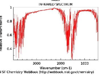
Fig. 1-2: Small portion of the absorption-emission spectrum of water vapour (NIST)
At first approximation, band models were developed to deal with portions of the spectrum at once rather than individual lines. The accuracy depends much on the spectral resolution, hence for this family of models one may distinguish the narrow band (higher resolution, Fig. 1-3) and wide band (lower resolution, Fig. 1-4) approaches, which both simplify the spectral dependency in a considerable way. Still, they mostly remain too involved for CFD applications, at least if the goal is to perform coupled calculations of the radiation and reactive flow fields. For decoupled calculations, narrow band approaches such as the statistical narrow band (SNB) and the narrow band correlated-k (NBCK) methods provide a good compromise between accuracy and computational time in fire conditions [9]. Wide band models like the exponential wide band (EWB) are more practical and can retain some spectral information, but in their spectral form they remain too expensive for many CFD applications, and may not directly yield absorption coefficients [10] (the RTE can be formulated in terms of transmissivity rather than absorption coefficients, but many CFD solvers use the latter formulation).
23
experienced major developments in recent years; however they are still not suitable for coupled simulations in large scale CFD applications due to relatively high computational costs (although progress has been recently reported in [13]). These methods contrast with the very crude grey approximations (single constant absorption coefficient for the whole spectrum), which are fastest but generally lead to poor predictions in combustion applications [14]. Alternatively to just one grey gas, several grey gases can be combined to reconstruct the total (spectral-integrated) properties of a real gas. Such is the approach of the weighted-sum-of-grey-gases (WSGG) [15], which curve-fits the total emissivity (spectral-integrated) of a real gas with polynomials. The polynomial coefficients are the radiative properties of a few fictitious grey gases, determined for certain conditions of temperature and concentrations. The total emissivity is determined beforehand, from a band model or measurements or both combined, hence the WSGG involves no actual spectral data. This flexible, fast, and easy to implement method is popular in CFD codes, but its accuracy is debated in the radiation literature (see next chapter). Also, due to its lack of spectral information the WSGG cannot be coupled with another non-grey phase (e.g. water droplets).
Fig. 1-3: Narrow band modelling of the 4.3µm rotation-vibrational region of CO2 (reproduced from [7])
24
1.2. Radiative properties of particulates in fires or fire suppression
Besides the gas phase, the presence of particulate media like soot (present in most fires and responsible for flame luminosity) or the liquid water droplets from a quenching system such as sprinklers or water sprays can radically alter the radiative properties of fires. Particulate media introduce radiative scattering [7], a group of three non-grey phenomena which describe the possible interactions between a particle and an incident ray: diffraction (ray deviated without contact), reflection (ray deviation after contact) and refraction (like reflection, with partial absorption). Depending on the new direction of the scattered ray, scattering can contribute positively or negatively to radiative intensity. The Mie theory describes the ensemble of these behaviours in a general way, by calculating the amplitudes of the electric and magnetic fields that constitute electromagnetic radiation. This model is thus very rigorous, but also very complex. Mie theory is advantageously replaced with simpler methods in some cases.
The soot particles usually produced by hydrocarbon fires are small enough to fall under the Rayleigh limit which treats the particulate phase as continuous. In this case the radiative properties of soot particles are described by their volume fraction [17]. As a further simplification, unlike in molecular gases the soot absorption spectrum is continuous (no transparent windows), and it is possible under certain conditions to use a Planck (grey) approximation with good accuracy [18,19]. The Rayleigh approach is however not valid for larger, coal-like soot particles for which Mie theory must be considered. Liquid droplets such as found in water sprays also require Mie modelling. The radiative properties of droplets change importantly with particle size; even if a monodisperse distribution is initially injected into the fire, droplets characteristics will change as a result of heat transfer. Moreover, heated-up droplets eventually evaporate, thus completely changing the gas mixture and its absorptive properties, and then it all changes again as temperature decreases. This problem has not yet been investigated in CFD.
1.3. Motivation, aims & objectives and contribution of the thesis
25
provide a good accuracy/computing times compromise. In the fire suppression scenario, the absorption coefficients of the liquid and gaseous phases are both non-grey. Hence to be added in the RTE, both phases must use the same spectral intervals. Since the WSGG gas model does not retain the physical information on the actual absorption bands of the gas, a wide band based box model is adopted in the current thesis to handle fire suppression scenarios involving gases and water droplets. The exponential wide band (EWB) model uses a small number of bands in each gas species (CO2, H2O, etc.). In each band an averaged absorptance is calculated, from which one can extract an absorption coefficient averaged over an equivalent bandwidth. This method, called the box model, or stepwise-grey wide band model [21], offers significant computational gain from the spectral formulation of the EWB, since for each band the absorption coefficient has a single average value instead of being a continuous function of wavenumber, which is analogous to a grey gas in WSGG. However unlike the WSGG, a box model relies on the assumption of an isothermal and homogeneous medium, hence to fit the inhomogeneous conditions of fires it must be scaled with a Curtis-Godson type method. Also, a box model may work with different band limits than the Mie theory model for water droplets.
The WSGG and EWB-box models were pioneered decades ago and have been improved over time. There are many WSGG correlations in the literature, obtained from older and newer spectral databases, developed for specific applications. However their accuracy in the particular context of pool fire CFD have been seldom assessed - at least some of the newest models have not been, to the best of this author's knowledge. Moreover, the works that did perform such studies have undertaken decoupled radiation/fluid flow approaches, whereas this work is aiming for an assessment in fully coupled simulations. For the box model, there are equally as few works available in the pool fire context, and on the topic of fire suppression, it is almost certain that the coupling of a box model with a Mie theory has not been attempted before. Hence the current work will make an important contribution not only to the growing community of FireFOAM users, but to the fire community in general.
In the thesis, five WSGG models (three banded, and two grey) and three box models (two with variable band limits, and one with fixed bands) have been implemented and investigated by this author in FireFOAM version 2.2.x for fire applications. The Mie theory model was implemented by FM Global at the same time and tested for liquid-only radiation scenarios. Eventually, in the last phases of this project the fixed bands box model was coupled with the Mie model in the developing version FireFOAM-dev available on the Github platform (https://github.com/firefoam-dev).
1.4. Layout of the thesis
26
27
Chapter 2 - Literature review
This chapter presents an overview of the literature available on the solution methods of the radiative transfer equation (RTE), the weighted-sum-of-grey-gases (WSGG), the exponential wide band (EWB) and box models, and radiation modelling in pool fires.
2.1. Overview of solution methods for the radiative transfer equation (RTE)
The RTE is a first-order difference equation with an integral term. If radiative heat transfer is considered instantaneous (an electromagnetic wave propagates at the speed of light), the transient term may be neglected and the general form of the RTE may be written as:
( , ) ( , ) =
−( + ) ( , ) + ( , ) , ( ) + ∫ ( , ) ( , ) ′ (2.1)
This equation has three dependencies of space and one of solid angle. The wavelength subscript denotes Eq. (2.1) may be solved for a single wavelength, or band, or the entire spectrum, depending on the spectral modelling strategy. An RTE solver thus generally discretises the spatial and/or angular domains, leaving the spectral properties to a sub-model. For heat transfer engineers, the interest is usually less in spectral information than in total properties such as the radiative heat flux or its divergence. To obtain these, it is not always mandatory to use an actual RTE solver. For example, a constant radiative fraction may be inputted by the user to yield the radiative source term trivially [22]; or an optically thin approximation (OTA) may directly yield the source term, assuming that the gas medium has a weak propensity to self-absorption, which means most of the radiative energy escapes to the surroundings [23]. In the opposite case, at the optically thick limit where self-absorption is strong, the P1 model assumes diffusive radiation where spherical harmonics replace the directional dependence of the RTE. Although the RTE is transformed into a second order difference equation this method saves significant computational time [24]. These fast methods contrast with the massive computational demands of the Monte-Carlo (MC) or ray tracing (RTM) methods based on statistical tracking of photons, which are thus more recommended for decoupled RTE calculations.
28
phenomenon, also called false scattering, is thus responsible for the increase of RE when working with grid refinements (commonplace in CFD). Hence angular and spatial grid size should be increased simultaneously, which can lead to a much increased computational effort. The work to eliminate RE from CFD simulations with the DOM or FVM is ongoing and some methods have been proposed in [26-28], where alternative angular discretisation schemes are proposed to avoid direct grid increases. RE elimination is a separate area of work to gas radiation modelling, but throughout this thesis RE will be briefly mentioned when needed as they can greatly affect the quality of prediction of the radiative heat flux. FVM theory will be summarised in the Mathematical Modelling chapter as well.
2.2. The weighted-sum-of-grey-gases (WSGG) model
Hottel and Sarofim developed the WSGG method [15] to reproduce their own measurements of total emissivities and absorptivities with polynomial curve fits. The method evolved both with band models and spectroscopic techniques, as both could be combined to overcome each other's shortcomings. In the early 1980s Smith et al. released their well-known WSGG correlations obtained from the EWB model [29]. For a long time the WSGG was used like a grey model, since it is easy to obtain a grey equivalent absorption coefficient from Beer's law, if a mean beam length can be determined. Later on, in the early 1990s Modest [30] showed that the WSGG could be used to solve the RTE for each grey gas individually, giving way to the non-grey WSGG implementation. This method increases the computational time from the grey version but it has the advantage of avoiding mean beam length approximations. Soufiani and Djavdan [31] used the non-grey formulation, generated WSGG correlations from an accurate statistical narrow band model (SNB) and compared both in a furnace-like scenario. In the last few years, some WSGG correlations based on up-to-date spectral data and narrow band modelling have been developed for oxy-fuel combustion, as in Cassol et al. and Johansson et al. [32,33]. These two newer models have been very recently tested in oxy-fuel conditions by Kez et al. [55], where large differences were noticed, while the older correlations from Smith et al. [29] were deemed unreliable even for qualitative analysis. The Cassol and Johansson WSGG models have however not yet been assessed for fire applications, which is a knowledge gap this work will attempt to address.
29
in [34] are not necessarily representative of fire conditions, and iii) newer WSGG correlations than those employed in [35] may have given different results. On the other hand, it is true that a WSGG cannot ever be expected to be as accurate as an SNB model, but it could be used with confidence if its errors in typical fire scenarios were quantified, as proposed in [37]. Hence the idea for this work of implementing the older Smith et al. model, and the newer WSGGs by Cassol et al. [32] and Johansson et al. [33] for a comparative study in fire conditions with a CFD finite volume radiation solver. These models will be described in more detail in the next chapter.
2.3. Exponential wide band (EWB) and box models
The EWB model was developed in the 1960s by Edwards [38]. By 1970, it had been extended for non-isothermal or inhomogeneous media, notably by Chan and Tien [39] or Cess and Wang [40], and in 1975 Felske and Tien proposed a method to remedy the band overlap problem [41]. The treatment of the pure rotational band of water vapour was refined by Modak in 1978 [42]. While spectral databases were not as developed as they are nowadays, the EWB model was deemed accurate enough to generate WSGG coefficients (e.g. Smith et al. [29]), and there are examples of that exercise even recently, e.g. in [43]. The box model, first proposed by Penner [44], is a stepwise-grey (spectrally coarser) version of the EWB. Unlike what Soufiani of Djavdan [31] observed with the WSGG (previous section), Modest and Sikka noticed that the box model performs better for a colder gas absorbing radiation emitted by hot walls, than the other way around [45]. Elsewhere, Nilsson and Sundén noticed an important sensitivity of EWB parameters to path length in [46]. This later issue will be investigated exhaustively in this work. On computational efficiency, several studies aimed at speeding up the EWB as CFD applications started in the 1990s, notably Lallemant and Weber [47] who greatly simplified some of the more tedious aspects of the original EWB formulation. Multidimensional applications of the EWB/box model also appeared around that time, e.g. in [45] where the P1 model was used with the banded EWB formulation (stepwise-grey absorption coefficient, as opposed to the smooth absorption coefficient of the spectral EWB). By the mid-1990s, there are examples of coupled radiation and convective heat transfer calculations, but without combustion, using spectral or box model versions of the EWB with a P1 approximation, see for instance the works of Seo et al. [48], Nilsson and Sundén [49] or Kaminsky et al. [50]. Seo et al. notably used a Curtis-Godson scaling technique to account for inhomogeneous gas radiation but reported accuracy issues for strong temperature and concentration gradients. In a related study, an early example of EWB (and narrow band) calculations in fires was from Komornicki and Tomeczek [51] who constructed a synthetic 750kW natural gas flame from experimental measurements, hence performing decoupled calculations in the inhomogeneous gas and (non-scattering) soot mixture. Such works however predate the era of modern CFD software with finite volume methods.
2.4. WSGG and EWB/box models in CFD codes and fire simulations
30
CFD fire simulations where the radiation and flow fields are coupled. In 2004 Snegirev [52] compared grey and banded WSGG implementations in 30cm propane pool fires, coupling a Monte-Carlo (MC) RTE solver with a RANS approach and including a simplified turbulence-radiation interaction (TRI) correction. Overall the banded WSGG tended to reduce the over-prediction of radiant fluxes, consistently with the pure-radiation works from [34-36]. In 2005, Dembele et al. [37] tested a banded formulation of an older WSGG model by Truelove within the frame of RANS CFD. While neglecting the turbulence-radiation interaction (TRI) they achieved good overall agreement between the predicted temperatures using the WSGG and the benchmark SNB data. Some CFD studies have employed and investigated other gas radiation models (e.g. SNB, NBCK, FSCK) by either coupling or decoupling the radiation and flow fields in jet flames [53]. Few recent works have investigated the effects of various gas models in oxy-fuel combustion [54-55]. On the EWB, an early CFD study (1998) is due to Cumber et al. [56] who performed a fully coupled RANS CFD jet flame simulation with both a spectral and a banded implementation of the EWB model. Among their conclusions, they i) underlined the superior accuracy of the spectral EWB over the banded implementation in the highly inhomogeneous, non-isothermal flame, and ii) remarked that radiation predictions were reasonably but not overly impacted by the errors on temperature and specie fractions resulting from the combustion model. Nilsson and Sunden [49] did a CFD simulation of bio-fuel combustion using the EWB and P1, solving the momentum equation but not the specie fractions [49], concluding that radiation in that case was more driven by the soot volume fraction. Nilsson et al. followed that in 2003 by showing how to optimise the EWB formulation for faster CFD calculations [46], resulting in two box models which turned out to be at least ten times faster than the regular EWB formulation, but become very sensitive to mean beam length approximations. Cumber and Fairweather [57] again tested a spectral EWB implementation in CFD studies of flames with a discrete transfer method (DTM), remarking that the radiation and combustion fields had different cell size requirements, which may cause problems [57]. Hostikka et al. [58] performed wide band modelling of various methanol and methane flames with Fire Dynamics Simulator (FDS, a LES CFD code with a FVM radiation solver), with Planck-averaging of the absorption coefficient in each band. Their predicted radiative fluxes were at times significantly larger than their experimental measurements, and they attributed the error to temperature overprediction from the combustion model while stressing the necessity to separate the error sources. More recently, coupled CFD simulations of 30cm methanol, heptane and toluene fires with FireFOAM were published by Chen et al. [23,59] and Chaterjee et al. [18], which relied on grey gas and/or grey soot modelling. The total radiative fractions approached the experimental values of [4] but the radiative fluxes to the flame surroundings were not reported.
31
vapour radiation near the pool surface. Recently Consalvi and Liu [6] compared approximate gas radiation models for idealised methane fires with FDS, several variants of the CK method and a stepwise-grey wide band model (similar to [58]) which performed poorly in the fuel rich core. Another decoupled method consists of reconstructing the temperature, gas species and soot fields from scaling techniques, such as McCaffrey's correlations [60], thus creating a synthetic pool fire. Krishnamoorthy [61] recently used that method combined with the experimental data of [4] to construct synthetic 30cm heptane and toluene fires. A comparison was made for grey and non-grey implementations of the EWB, (Smith et al.'s [29]) WSGG, SLW and RADCAL coupled with a DOM solver. The results show that the solution method (grey or non-grey) has more influence on the radiant flux and source term than the model itself. The same 30cm toluene fire was further investigated by Consalvi et al. [19] who used an accurate SNBCK model with the FVM. They studied the separate influences of TRI/no TRI and banded/grey soot treatments with normal and lighter (more heptane-like) soot loadings. The neglecting of TRI resulted in an important decrease of the radiative heat flux and source term, whereas the error induced by the grey soot modelling was visible but not as important (the grey soot model was acceptable for the lighter soot loading). Consalvi et al.'s radiant flux at the pool surface held comparison with the experimental values of [4], however Krishnamoorthy's fluxes are largely underpredicted [61], despite also using a TRI correction. On the issue of TRI, Coelho issued exhaustive reviews in [62,63] and recommended the use of different types of correlations depending on the optical thickness. Among the works listed here, however, TRI corrections were often neglected (mentions of implemented TRI in [18,19,52,53,61] but not in [5,6,37,56,58,59]).
With the relative rarity of WSGG or EWB box model usage in pool fires, it is worth mentioning some recent CFD works in oxy-fuel combustion, such as Marzouk and Huckaby [64] who implemented an EWB/box model in ANSYS Fluent 13 and carried out radiation calculations for gas mixtures at typically high CO2 and H2O gas mole fractions with grey walls. The many band overlaps induced by the high mole fractions of each specie resulted in box model spectra of 20+ bands (CO2 and H2O have only 6 and 5 bands in the EWB). They however include detailed data of their box model absorption spectra calculations which may come useful to verify our own box model implementations. EWB and box models for oxy-fuel and furnace combustion are also studied within the last decade by Stefanidis et al. [65] (coupled convective and radiative heat transfer, but non-reactive flow).
2.5. Fire suppression by water sprays
32
33
Chapter 3 - Mathematical modelling
3.1. Governing equations
The Navier-Stokes equations are briefly outlined here, in their averaged form suitable for the large eddy simulation (LES) approach. The over-bars and tildes stand for spatial filtering and Favre averaging respectively.
Mass:
+ = 0 (3.1)
Momentum:
+ = ̅ + ̅( + ) + − + ̅ (3.2)
( , , = 1,2,3) , = 1 =
0 ≠
Gas species:
+ = ̅ + + , + , + , (3.3)
( = , , , )
Soot:
+ = ̅ + + , + , (3.4)
Sensible enthalpy - Energy:
+ = ̅+ ̅ + + ̇ − ∇. ̇ ′′ (3.5)
ℎ = ∫ ∑ ( ) (3.6)
= + . ∇ (3.7)
̇ = , ℎ − , ℎ , (3.8)
Where -∇.q''r is the divergence of the radiative flux, or radiative source term, or radiative power dissipated per unit volume. This last term is responsible for the coupling of radiation energy expressing the conservation of total energy. At a spatial location x and time t the radiative source term is expressed as:
34
Where s is the direction vector of the unit solid angle d through which the monochromatic radiative intensity Iλ propagates. Iλ is the solution of the radiative transfer equation [76].
3.2. The general radiative transfer equation
3.2.1. Blackbody intensity
A blackbody is an idealised object that perfectly absorbs and re-emits radiation at any wavelength. Thus continuous, the spectrum follows Planck's distribution. The monochromatic intensity of a blackbody at equilibrium temperature T is given by the law of Planck [76]:
, ( , , ) =
( , )
e
( , )
− 1 = ( , ) , ( ) (3.10)
Where , ( ) is the isotropic blackbody intensity in vacuum (superscript 0). The velocity of electromagnetic wave propagation in the medium, c, depends on the real part of the medium's complex index of refraction, i.e. n(x,s) = c0/c(x,s) is the isotropic blackbody intensity in vacuum.
3.2.2. Radiative heat flux
The elementary flux of the elementary ray propagating at position x, inside d and normally to the elementary surface dS (Fig. 3-1) may be defined as [76]:
= (3.11)
Where Iλ is the intensity at position x and may or may not be at radiative equilibrium. The variation of , for a small displacement dx along the path length, is:
= ( + ) − ( ) (3.12)
Clausius' relation of conservation yields:
( + ) ( + ) ( + ) = ( ) ( ) (3.13)
The flux of Eq. 3.11 can be redefined as:
( ) = ( ) ( ) ( ) ( ) (3.14)
Hence:
( ) = ( ) ( + ) ( + ) ( + ) (3.15)
Writing Eq. 3.14 for x + dx and subtracting Eq. 3.15, the variation of the flux is:
35
[image:36.595.214.408.131.294.2]Where dV = dSdx, and the thermal radiative capacity was considered negligible compared with the thermal material capacity, which underlies the instantaneity of the propagation of radiation compared with the other heat transfer modes.
Fig. 3-1: Optical path between two arbitrary points in an arbitrary medium (reproduced from [76])
3.2.3. Absorption and spontaneous emission
The flux absorbed by the volume dV between two positions must be proportional to that volume, the solid angle, the spectral interval and the incident intensity:
= (3.17)
Where is the monochromatic absorption coefficient (m-1). The medium is also characterised by its monochromatic emission coefficient ξλ(x), defined as:
= (3.18)
At thermal equilibrium, the intensity in all directions and at any position is ( , ) , ( )
as defined earlier by the law of Planck. If the equilibrium is stable or near stable, the emitted flux is equal to the absorbed flux, hence the monochromatic emission coefficient ξλ(x) can be expressed from Eq. 3.17 and 3.18 as:
= ( , ) , ( ) (3.19)
Which yields the flux emitted by the medium inside the volume dV and solid angle d:
= ( , ) , ( ) (3.20)
3.2.4. Scattering
36
solid angle d (Fig. 3-2). The first case, subscripted d-, is analogous to absorption, hence it
can be characterised by a monochromatic scattering coefficient σλ (also in m-1) defined by:
= (3.21)
In the second case, let s' be the initial direction of the ray reaching position x and s the new direction of the ray exiting at x+dx. The ray scattered in a random direction is ′ . The probability P for the incident flux to scatter within d must depend on a phase function ( ′, ) veryfying:
= ( ′, ) (3.22)
The flux coming from all directions and scattered constructively by the volume dV inside the solid angle d, is defined by:
= ∫ ( , ) ( ) ′ (3.23)
Fig. 3-2: Radiative scattering from unit volume dV (reproduced from [76])
3.2.5. Energy conservation
Finally, the radiative transfer equation (RTE) is constructed from the terms defined above. If the flux variation though dV (Eq. 3.16) is the sum of the absorbed flux (Eq. 3.17), the emitted flux (Eq. 3.20) and the two flux contributions due to scattering (Eq. 3.21 and 3.23), then the RTE takes the form:
( , ) ( , ) =
−( + ) ( , ) + ( , ) , ( ) + ∫ ( , ) ( , ) ′ (3.24)
3.3. Non-scattering media
37
the integro-differential term from Eq. 3.24, and the scattering coefficient which, with the absorption coefficient, contributes to extinction. The RTE reduces to an ordinary difference equation with constant term (i.e. blackbody radiation is only a function of temperature, which is always known locally in the simulation):
. ∇ ( , ) = ( , ( ) − ( , )) (3.25)
Where κλ is the linear monochromatic absorption coefficient (m-1). The radiative source term defined in Eq. 3.9 may now be rewritten as:
−∇. ̇ ′′ = ∫ 4 , − ∫ (3.26)
The total radiant power dissipated through a volume by a source can be obtained by a volume integration of the source term, but also by a surface integration of the flux at radiative equilibrium (q''net =q''incident-q''background) since the flux must verify the divergence theorem.
3.4. Solutions of the non-scattering RTE
The non-scattering spectral RTE (Eq. 3.25) is solved along a line of sight, or optical path. At a distance L from the origin, if the medium between 0 and L is isothermal and homogeneous, then an analytical solution is given:
( ) = (0) + , (1 − ) (3.27)
Where the non-dimensional product is the optical thickness of the medium at wavelength λ. An absorption line with >> 1 is opaque, respectively transparent if << 1. The quantity is the spectral transmissivity, or Beer's law, expressing the decrease of radiative energy as it traverses the absorbing medium. In the general case of an inhomogeneous or non-isothermal medium Beer's law generalises to:
= ∫ ( ) (3.28)
In Eq. 3.28 the integration of the optical depth between the origin and the optical path is only possible along a line of sight. CFD solvers which deal with multidimensional problems must adopt an approximation called the uncorrelated method. Rewriting the exact (correlated) solution of Eq. 3.27 in terms of transmissivity, for a path discretised in i elements between 0 and n, yields [33]:
, = , , → + ∑ , , / , → − , → (3.29)
The uncorrelated solution retains history only from the previous neighbouring cell:
, = , , + , , / 1 − , (3.30)
38
coefficient, but a grid dependency may be introduced in inhomogeneous media. For gas radiation models where a path length is required to calculate the absorption coefficient, the mean beam length (MBL) is a common approximation.
3.5. Mean beam lengths
First developed by Hottel [7], the idea is that from the perspective of an elementary black surface, there is no difference whether incident radiation is coming from all directions within a hemisphere or a distant emitting object, hence a certain hemisphere radius R can be defined such as R is equal to a mean beam length S (Fig. 3-3). MBL are usually not trivial to calculate directly and are distinguished between geometrical MBL and spectral-averaged MBL. Geometrical MBL are calculated at the optically thin limit, where energy escapes easily from the medium to its (black) surroundings. The geometric MBL is defined by S0 = 4V/A, where V and A are the volume and area of the radiating medium. Spectral-averaged MBL, on the other hand, rely on Hottel's observation that the spectral radiative flux is not very sensitive to the spectral fluctuations of S, hence the MBL can be made independent from the spectral absorption coefficient with reasonable accuracy [7]. Further empirical observations have confirmed that the ratio between the spectral-averaged and geometric MBL is close to 0.9, hence the spectral-averaged MBL may be written as:
≈ 0.9 = 3.6 / (3.31)
In [7] Modest gives a table of MBL for various geometries. The MBL is easy to calculate for e.g. participating media entirely filling an enclosure of simple geometry, or a 1D slab of thickness L (in which case S = 1.8L). It is less easy in the case of a pool fire (the methods from this author and others' works will be discussed in the dedicated chapter), and it gets further more difficult for freely spreading fires whose shapes are irregular and change with time. Even with just pure radiation inside 2D or 3D box scenarios, the MBL method may introduce errors (see next chapter).
Fig. 3-3: Isothermal gas volume radiating to surface element for (a) an arbitrary gas volume, and (b) for an equivalent hemisphere radiating to the centre of its base where Le
39
3.6. Angular and Spatial discretisation of the non-scattering RTE
The finite volume (FVM) method is the mathematical tool of choice for solving most equations in OpenFOAM, hence in FireFOAM, such as the Navier-Stokes equations (Eq. 3.1-3.8 above). The P1 and optically thin approximation methods are available in FireFOAM, giving direct access to the radiative source term without actual solution of the non-scattering RTE (Eq. 3.25) but these ready solutions only work for the optically thin and optically thick limits, whereas the FVM is for any thickness. Called "fvDOM" in the code, the method integrates Eq. 3.25 over the computational cell volume Vijk and solid angle l, respectively expressed in Cartesian and spherical coordinates. For the latter, the polar angle θ is between the z axis and the xy plane, and the azimuthal angle φ is between the x and y axes. Subdivisions in each angular direction determines l, portion of the total solid angle equal to 4π. Eq. 3.25 thus becomes:
∫ ∫ . ∇ ( , ) = ∫ ∫ ( )( , ( ) − ( , )) (3.32)
The divergence theorem can be used to replace the volume integration on the left side with a surface integration on all 6 faces. Assuming the intensity is equal on each face, the integral can be replaced with a summation. Also, if the intensity is constant inside Vijk and on the solid angle l, then:
∑ , ∫ ( . ) = , , , − , (3.33)
Where , is the monochromatic intensity in the direction l, , the intensity on the face
m, the solid angle corresponding to direction l, the area of the face m, nm the unit vector normal to face m. , is calculated with a Gauss linear upwind, second order scheme. To provide closure, the following boundary condition is used, where walls are assumed to be diffusive but can be nonblack (i.e. partially reflective):
, = , , , + , ∑ , (3.34)
Where
= ∫ ( . ) (3.35)
The first term on the right hand side of Eq. 3.34 is the intensity emitted by the wall, where
ελ,w is the monochromatic wall emissivity, i.e. the ratio of the energy emitted by the surface over the energy emitted by a blackbody at the same temperature, both integrated over all directions of space. The wall emissivity is sometimes called emittance to avoid confusion with the gas emissivity, defined in the next section. If the wall is black (ελ,w = 1), the reflective term (second-right) cancels out. nw is the unit vector normal to the wall. The constraint
< 0 means that only the directions incident to the wall are considered in the reflective
40
3.7. Weighted-sum-of-grey-gases (general formulation)
The WSGG is a relatively simple but powerful way of modelling the total radiative properties of a gas. From the spectral transmissivity (Eq. 3.28), the spectral emissivity ελ and spectral absorptivity αλ are defined as:
(0 → ) = (0 → ) = 1 − = 1 − ∫ ( ) (3.36)
The total emissivity and total absorptivity are obtained by spectral integration, but then they are no longer rigorously equal since they have different temperature dependencies. Total emissivity thus depends only local gas temperature:
( , ) =
( )∫ 1 −
∫ ( ( ))
, (3.37)
Whereas the total absorptivity:
( , , ) =
( )∫ 1 −
∫ ( ( ))
, ( ) (3.38)
Where T can be either the gas temperature Tg or the wall temperature Tw [7]. Hence, the total absorptivity depends on the spectral structure of the incident radiation intensity and cannot be tabulated in a general way (to quote Soufiani and Djavdan in [31]). In a pool fire, the more likely radiation scenario is that the medium is a net emitter to colder boundaries. The emissivity-formulated WSGG is thus more likely to work better for fires; also, WSGG models like those of Cassol et al. [32] and Johansson et al. [33] are only formulated in that manner. The total emissivity is then approximated by a weighted sum of grey gases:
( , ) = 1 − ≈ ∑ ( ) 1 − (3.39)
41
3.7.1. Grey WSGG formulation
Once the approximate total emissivity is calculated, Eq. 3.39 easily yields the grey absorption coefficient:
( , ) = − ( , ) (3.40)
Eq. 3.25 thus becomes:
. ∇ ( , ) = ( )[ ( ( )) − ( , )] (3.41)
Which may be solved for each solid angle. The term = / is the total blackbody energy. The finite volume solution of Eq. 3.41 yields the total directional intensity (W/m²/sr), which is integrated over the solid angle to yield the total incident radiation G (W/m²):
( ) = ∫ ( , ) (3.42)
From which the total radiative source term is obtained (where the absorption coefficient and blackbody intensity may vary locally if the gas is inhomogeneous and/or non-isothermal):
∇. ̇ ( ) = ( )[4 ( ) − ( )] (3.43)
The total radiative flux incident to a boundary with normal unit vector nw is:
̇ , ( ) = ∫. ( , )| . | (3.44)
3.7.2. Banded or non-grey WSGG formulation
While computationally attractive, the "grey" WSGG method is not necessarily the most accurate, due to the averaging over the mean beam length of Eq. 3.40 and the non-rigorous validity of the Beer law for total emissivity. Also, as said before the mean beam length can be difficult to evaluate for some fires. As an alternative to that, Modest [30] proposed a non-grey (banded) formulation of the WSGG method , showing that the kj and aj could be used directly in gas-by-gas solutions the RTE (thus solved J times in each direction). The total intensity, solution of the total non-scattering RTE may be expressed as a function of total emissivity:
( ) = , [1 − ( , 0 → )] − ∫ [ ( ), → ] ( ) ′ (3.45)
Substituting Eq. 3.39 into 3.45 leads to:
( ) = ∑ , + ∫ ∑ ( ) ′ = ∑ +
42
By identification, the total intensity is thus simply the summation on all grey gas intensities:
( ) = ∑ ( ) (3.47)
Which finally verifies the RTE for an individual grey gas:
. ∇ = ( ) ( ) − (3.48)
With the following boundary condition for a diffusive black wall:
, = ( ) ( ) (3.49)
Note that Eq. 3.49 is simply the black (non-reflective) version of Eq. 3.34. The mean beam length approximation is now altogether bypassed. To calculate the incident radiation G and incident flux q''r,in, Eq. 3.47 is simply injected in Eq. 3.42 and 3.44. However the source term (Eq. 3.43) now takes this form:
∇. ̇ ( ) = ∑ ( ) ( ) 4 ( ) ( ) − ∑ ( ) , ( , ) (3.50)
Where i is the ith solid angle. The original FireFOAM code for the finite volume solver (fvDOM) was modified accordingly to accommodate for banded RTE solutions involving the WSGG weighting coefficient. This was done by adding the temperature-dependent weighting factor in the expression of blackbody intensity in the Radiative Intensity Ray and fvDOM classes. The expression of the source term or radiant flux divergence was also modified in fvDOM so that the incident radiation is directly factored by the band or grey gas absorption coefficient, upon each iteration of the band loop. The incident radiation itself is now calculated and stored for each band, and likewise for the boundary fluxes (incident, emitted, net) in the fvDOMclass and the Wide Band Diffusive Radiation (boundary condition). The total fluxes are reconstructed during post-processing by simply adding the contributions from each band. These modifications work with a banded WSGG or any other band model (where the WSGG weighting factor may be replaced by the physical Planck function).
3.8. The three sets of WSGG correlations implemented in FireFOAM
43
[image:44.595.105.489.186.445.2]Smith et al.'s WSGG parameters for emissivity are listed as follows in Table 3-1, for small amounts of CO2, small and large amounts of H2O and two H2O-CO2 mixtures. They are valid for temperatures between 600 and 2400K, and pressure-path lengths between 10-3 and 10 atm.m. The pressure absorption coefficients kj are in (atm.m)-1 and the emissivity factors bi,j are in powers of temperature.
Table 3-1: Emissivity correlations for Smith et al.'s WSGG model [29]
j kj bj,1.101 bj,2.104 bj,3.107 bj,4.1011
CO2 (pc->0)
1 0.3966 0.4334 2.62 -1.56 2.565
2 15.64 -0.4814 2.822 -1.794 3.274
3 394.3 0.5492 0.1087 -0.35 0.9123
H2O (pw->0)
1 0.4098 5.977 -5.119 3.042 -5.564
2 6.325 0.5677 3.333 -1.967 2.718
3 120.5 1.8 -2.334 1.008 -1.454
H2O
(pw=1atm)
1 0.4496 6.324 -8.358 6.135 -13.03
2 7.113 -0.2016 7.145 -5.212 9.868
3 119.7 3.5 -5.04 2.425 -3.888
PW/PC = 1
1 0.4304 5.15 -2.303 0.9779 -1.494
2 7.055 0.7749 3.399 -2.297 3.77
3 178.1 1.907 -1.824 0.5608 -0.5122
PW/PC = 2
1 0.4201 6.508 -5.551 3.029 -5.353
2 6.516 -0.2504 6.112 -3.882 6.528
3 131.9 2.718 -3.118 1.221 -1.612
The non-dimensional temperature dependent weight for a grey gas is given by:
( ) = ∑ , (3.51)
The fourth "band" is a clear gas meant to account for all the windows in the real gas' spectrum, hence k4 is always zero and a4 must verify:
= 1 − ∑ (3.52)
![Fig. 3-1: Optical path between two arbitrary points in an arbitrary medium (reproduced from [76])](https://thumb-us.123doks.com/thumbv2/123dok_us/9434081.450005/36.595.214.408.131.294/fig-optical-path-arbitrary-points-arbitrary-medium-reproduced.webp)
![Table 3-1: Emissivity correlations for Smith et al.'s WSGG model [29]](https://thumb-us.123doks.com/thumbv2/123dok_us/9434081.450005/44.595.105.489.186.445/table-emissivity-correlations-smith-et-al-wsgg-model.webp)
![Table 3-4: Exponential wide band model coefficients for H2O [7]](https://thumb-us.123doks.com/thumbv2/123dok_us/9434081.450005/49.595.67.564.370.638/table-exponential-wide-band-model-coefficients-h-o.webp)
![Table 3-5: Exponential wide band model coefficients for CO2 [7]](https://thumb-us.123doks.com/thumbv2/123dok_us/9434081.450005/50.595.68.576.95.329/table-exponential-wide-band-model-coefficients-co.webp)
![Fig. 4-1-7: (a), (b) Radiative source term along (x, yincident flux along ( = 0.25) and (x = 0.5, y), (c), (d) x, y = 0.5) and (x = 1, y) for the non-isothermal 2D enclosure of [35], FireFOAM-WSGG vs SNB of [35]](https://thumb-us.123doks.com/thumbv2/123dok_us/9434081.450005/70.595.91.525.78.411/fig-radiative-source-yincident-isothermal-enclosure-firefoam-wsgg.webp)
![Fig. 4-1-8: (a), (b) Radiative source term = 4m) for the 3D enclosure of [34], FireFOAM) and (= 1m, zx, y = 1, z = 3D enclosure of [34], FireFOAM-WSGG vs SNB of [34,84](d) incident flux along ((b) Radiative source term along (x = 2m, y = 1m, x = 1m, z) and (y = 1m, x, y = 1m, z) and (0.375m) ; (c), (d) incident flux along (WSGG vs SNB of [34,84]](https://thumb-us.123doks.com/thumbv2/123dok_us/9434081.450005/71.595.107.479.442.721/radiative-enclosure-firefoam-enclosure-firefoam-incident-radiative-incident.webp)
![Fig. 4-1-11: Comparison of FireFOAM-WSGG line-of-sight solutions with DBT-SNB from [36] for different soot volume loadings (non-isothermal, inhomogeneous)](https://thumb-us.123doks.com/thumbv2/123dok_us/9434081.450005/74.595.78.515.77.435/comparison-firefoam-solutions-different-volume-loadings-isothermal-inhomogeneous.webp)
