Unrestricted Quantifier Scope Disambiguation

Unrestricted Quantifier Scope Disambiguation

Mehdi Manshadi and James Allen

Department of Computer Science, University of Rochester

Rochester, NY, 14627, USA

{mehdih,james}@cs.rochester.edu

Abstract

We present the first work on applying sta-tistical techniques to unrestricted Quanti-fier Scope Disambiguation (QSD), where there is no restriction on the type or the number of quantifiers in the sentence. We formulate unrestricted QSD as learning to build a Directed Acyclic Graph (DAG) and define evaluation metrics based on the properties of DAGs. Previous work on sta-tistical scope disambiguation is very lim-ited, only considering sentences with two explicitly quantified noun phrases (NPs). In addition, they only handle a restricted list of quantifiers. In our system, all NPs, ex-plicitly quantified or not (e.g. definites, bare singulars/plurals, etc.), are considered for possible scope interactions. We present early results on applying a simple model to a small corpus. The preliminary results are encouraging, and we hope will motivate further research in this area.

1

Introduction

There are at least two interpretations for the fol-lowing sentence:

(1) Every line ends with a digit.

In one reading, there is a unique digit (say 2) at the end of all lines. This is the case where the quanti-fier A outscopes (aka having wide-scope over) the quantifier Every. The other case is the one in which

Every has wide-scope (or alternatively A has nar-row-scope), and represents the reading in which different lines could possibly end with distinct dig-its. This phenomenon is known as quantifier scope ambiguity.

Shortly after the first efforts to build natural lan-guage understanding systems, Quantifier Scope Disambiguation (QSD) was realized to be very difficult. Woods (1978) was one of the first to sug-gest a way to get around this problem. He pre-sented a framework for scope-underspecified semantic representation. He suggests representing the Logical Form (LF) of the above sentence as:

(2) <Every x Line>

<A y Digit> Ends-with(x, y)

in which, the relative scope of the quantifiers is underspecified. Since then scope underspecifica-tion has been the most popular way to deal with quantifier scope ambiguity in deep language understanding systems (e.g. Boxer (Bos 2004), TRAINS (Allen et al. 2007), BLUE (Clark and Harrison 2008), and DELPH-IN1_{). Scope} under-specification works in practice, only because many NLP applications (e.g. machine translation) could be achieved without quantifier scope disambigua-tion. QSD on the other hand, is critical for many other NLP tasks such as question answering sys-tems, dialogue systems and computing entailment.

Almost all efforts in the 80s and 90s on QSD adopt heuristics based on the lexical properties of the quantifiers, syntactic/semantic properties of the sentences, and discourse/pragmatic cues (VanLehn

1 _{http://www.delph-in.net/}

1978, Moran 1988, Alshawi 1992). For example, it is widely known that in English, the quantifier

each tends to have the widest scope. Also, the sub-ject of a sentence often outscopes the direct ob-ject.2 _{In cases where these heuristics conflict,} (manually) weighted preference rules are adopted to resolve the conflict (Hurum 1988, , Pafel 1997).

In the last decade there has been some effort to apply statistical and machine learning (ML) tech-niques to QSD. All the previous efforts, however, suffer from the following two limitations (see sec-tion 2 for details):

• They only allow scoping two NPs per sentence. • The NPs must be explicitly quantified (e.g. they

ignore definites or bare singulars/plurals), and the quantifiers are restricted to a predefined list. In this paper, we present the first work on applying statistical techniques to unrestricted QSD, where we put no restriction on the type or the number of NPs to be scoped in a sentence. In fact, every two NPs, explicitly quantified or not (including defi-nites, indefidefi-nites, bare singulars/plurals, pronouns, etc.), are examined for possible scope interactions. Scoping only two quantifiers per sentence, the pre-vious work defines QSD as a single classification task (e.g. 0 where the first quantifier has wide-scope, and 1 otherwise). As a result standard met-rics for classification tasks are used for evaluation purposes. We formalize the unrestricted form of QSD as learning to build a DAG over the set of NP chunks in the sentence. We define accuracy, preci-sion and recall metrics based on the properties of DAGs for evaluation purposes.

We report the application of our model to a small corpus. As seen later, the early results are promising and shall motivate further research on applying ML techniques to unrestricted QSD. In fact, they set a baseline for future work in this area.

The structure of this paper is as follows. Section (2) reviews the related work. In (3) we briefly de-scribe our corpus. We formalize the problem of quantifier scope disambiguation for multiple quan-tifiers in section (4) and define some evaluation metrics in (5). (6) presents our model including the kinds of features we have used. We present our experiments in (7) and give a discussion of the re-sults in (8). (9) summarizes the current work and gives some directions for the future work.

2 _{Allen (1995) discusses some of these heuristics and gives an}

algorithm to incorporate those for scoping while parsing.

2

Related work

Earlier we mentioned that a standard approach to deal with quantifier scope ambiguity is scope un-derspecification. More recent underspecification formalisms such as Hole Semantics (Bos 1996), Minimal Recursion Semantics (Copestake et al. 2001), and Dominance Constraints (Egg et al. 2001), present constraint-based frameworks. Every constraint forces one term to be in the scope of another, hence filters out some of the possible readings. For example, one may add a constraint to an underspecified representation (UR) to force is-land constraints. Constraints can be added incre-mentally to the UR as the sentence processing goes deeper (e.g. at the discourse and/or pragmatic level). The main drawback with these formalisms is that they only allow for hard constraints; that is every scope-resolved representation must satisfy all the constraints in order to be a valid interpreta-tion of the sentence. In practice, however, most constraints that can be drawn from discourse or pragmatic knowledge have a soft nature; that is, they describe a scope preference that is allowed to be violated, though at a cost.

Motivated by the above problem, Koller et al. (2008) define an underspecified scope representa-tion based on regular tree grammars, which allows for both hard constraints and weighted soft con-straints. They present a PCFG-style algorithm that computes the reading, which satisfies all the hard constraints and has the maximum product of the weights. However, they assume that the weights are already given. Their algorithm, for example, can be used in traditional QSD approaches with weighted heuristics to systematically compute the best reading. The main question though is how to automatically learn those weights. One solution is using corpus-based methods to learn soft con-straints and the cost associated with their violation, in terms of features and their weights.

list. This forms a corpus of 890 sentences, each labeled with the relative scope of the two quantifi-ers, with the possibility of no scope interaction. The no scope interaction case happens to be the majority class in their corpus and includes more than 61% of the sentences, defining a baseline for their QSD system. They achieve the inter-annotator agreement of only 52% on this task.

They treat QSD as a classification task with three possible classes (wide scope, narrow scope, and no scope interaction). Three forms of feature are incorporated into the classifier: part-of-speech (POS) tags, lexical features, and syntactic proper-ties. Several classification models including naïve Bayes classifier, maximum entropy classifier, and single-layer perceptron are tested, among which the single-layer perceptron performs the best, with the accuracy of 77%.

Galen and MacCartney (2004), hence GM04, build a corpus of 305 sentences from LSAT and GRE logic games, each containing exactly two quantifiers from an even more restricted list of quantifiers. They use an additional label for the case where the two scopings are equivalent (as in the case of two existentials). In around 70% of the sentences in their corpus, the first quantifier has wide scope, defining a majority class baseline of 70% for their QSD system.3 _{Three classifiers are} tried: naïve Bayes, logistics regression, and support vector machine (SVM), among which SVM per-forms the best and achieves the accuracy of 94%.

In a recent work, Srinivasan and Yates (2009) study the usage of pragmatic knowledge in finding the preferred scoping of natural language sen-tences. The sentences are all extracted from 5-grams in Web1Tgram (from Google, Inc) and share the same syntactic structure: an active voice English sentence of the form (S (NP (V (NP | PP)))). For the task of finding the most preferred reading, they annotate 46 sentences, each contain-ing two quantifiers: Every and A, where the first quantifier is always A. Each sentence is annotated with one of the two labels (Every has wide scope or not). They use a totally different approach for finding the preferred reading. The n-grams in Web1Tgram are used to extract relations such as

Live(Person, City), and to estimate the expected cardinality of the two classes, which form the ar-guments of the relation, that is Person and City.

3 _{They do not report any inter-annotator agreement.}

They decide on the preferred scoping by compar-ing the size of the two classes, achievcompar-ing the accu-racy of 74% on their test set. The main advantage of this work is that it is open domain.

3

Our corpus

The fact that HS03, in spite of ignoring challeng-ing scope phenomena and scopchalleng-ing only two quanti-fiers per sentence, achieve the IAA of 52% shows how hard scope disambiguation could be for hu-mans. It becomes enormously more challenging when there is no restriction on the type or the number of quantifiers in the sentence, especially when NPs without explicit quantifiers such as de-finites, indede-finites, and bare singulars/plurals are taken into account. As a matter of fact, our own early effort to annotate part of the Penn Treebank with full scope information soon proved to be too ambitious. Instead, we picked a domain that covers most challenging phenomena in scope disambigua-tion, while keeping the scope disambiguation fairly intuitive. This made building the first corpus of English text with full quantifier scope information feasible. Our domain of choice is the description of tasks about editing plain text files, in other words, a natural language interface for text editors such as SED, AWK, or EMACS. Figure (1) gives some sentences from the corpus. The reason behind scoping in this domain being fairly intuitive is that given any of these sentences, a conscious knowl-edge of scoping is critical in order to be able to accomplish the explained task.

Our corpus consists of 500 sentences manually extracted from the web. The sentences have been labeled with gold standard NP chunks, where each NP chunk has been indexed with a number 1 through n (n is the number of chunks in the sen-tence). The annotators are asked to use outscoping relations represented by ‘>’ to specify the relative scope of every pair 1≤i,j≤n, with an option to leave

1.Print [1/ every line] of [2/ the file] that starts with [3/ a digit] followed by [4/ punctuation].

QSD: {2>1, 2>3, 1>3, 2>4, 1>4}

2.Delete [1/ the first character] of [2/ every word] and [3/ the first word] of [4/ every line] in [5/ the file].

QSD: {5>4, 5>3, 4>3, 5>2, 5>1, 2>1}

the pair unscoped. For example a relation (2>3) states that the second NP in the sentence outscopes

(aka dominates) the third NP. Since outscoping relation is transitive, for the convenience of the annotation, the outscoping relations are allowed to be cascaded forming dominance chains. For exam-ple, the scoping for the sentence 2 in figure (1) can alternatively be represented as shown in (3).

(3) (5>2>1 ; 5>4>3)

As a result, every pair <i,j> (1≤i<j≤n) is implicitly labeled with one of the three labels:

i. Wide scope: either explicitly given by the annotator as i>j or implied using the transi-tive property of outscoping4

ii. Narrow scope: either explicitly given by the annotator as j>i or implied using the transi-tive property of outscoping

iii. No interaction: where neither wide scope nor narrow scope could be inferred from the given scoping.5

We achieved the IAA of 75% (based on Cohen’s kappa score) on this corpus, significantly better than the 52% IAA of HS03, especially considering the fact that we put no restriction on the type of the quantification. Our sentence-level IAA is around 66%. The details of the corpus, and the annotation scheme are beyond the scope of this paper and can be found in Manshadi et al. (2011).

4

Formalization

Outscoping is an anti-symmetrictransitive relation, so it defines an order over the chunks. Since we do not force every two chunks to be involved in an outscoping relation, QSD defines a partial order

over the NP chunks. Formally,

Definition 1: Given a sentence S with NP chunks

1..n, a relation P over {1..n} is called a QSD for S, if and only if P is a partial order.

Definition 2: Given a sentence S with NP chunks

1..n, and the QSD P, we say (chunk) i outscopes

(chunk) j if and only if (i>j) ∈ P.

4 _{That is if i outscopes j and j outscopes k then i outscopes k.} 5 _{The no interaction class includes two cases: no scope}

interac-tion and logical equivalence which means we follow the three-label scheme of HS03 as opposed to the four-three-label scheme of GM04. This is because when there is a logical equivalence, except for trivial cases, there are no clear criteria based on which one can decide whether there is a scope interaction or not. Furthermore, distinguishing these two cases does not make much difference in practice.

Definition 3: Given a sentence S with NP chunks

1..n, and the QSD P, chunk i is said to be disjoint

with chunk j if and only if

(i>j) ∉ P ∧ (j>i) ∉ P.

4.1

Partial orders can be represented using Directed Acyclic Graphs (DAGs) in which dominance (aka

reachability) determines the order. More precisely, every DAG G over n nodes v1..vn defines a partial

order PG over the set {v1..vn} in which, vi precedes

vj in PG if and only if vidominates6vj in G.

Definition 4: Given a sentence S with NP chunks

1..n, every DAG G over n nodes (labeled 1…n) defines a QSD PG for S, such that

(i>j) ∈ PG⇔ i dominates j in G

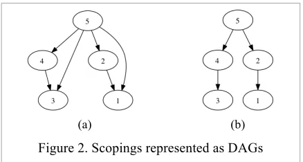
For example figure (2a,b) represent the DAGs cor-responding to the QSD of sentence 2 in figure (1) and the QSD in (3) respectively. Following defini-tion 3 and 4, the no interacdefini-tion reladefini-tion defined in section (3) translates to corresponding nodes in the DAG being disjoint7. Therefore the three types of scope interaction defined in i, ii, and iii (section 3), translate to the following relations in a DAG.

(4) Wide Scope (WS): i dominates j

Narrow Scope (NS): j dominates i No Interaction (NI): iand j are disjoint.

5

Evaluation metrics

Intuitively the similarity of two QSDs, given for a sentence S, can be defined as the ratio of the chunk pairs that have the same label in both QSDs to the total number of pairs. For example, consider the

6 _{Given a DAG G=(V, E), node u is said to immediately}

dominate node v if and only if (u,v) ∈ E. “dominates” is the

reflexive transitive closure of “immediately dominates”.

7 _{The nodes u and v of the DAG G are said to be disjoint if}

neither u dominates v nor v dominates u.

(a) (b)

two DAGs in figure (2). Although looking differ-ent, both DAGs define the same partial order (i.e. QSD). This is because the partial order represented by a DAG G corresponds to the transitive closure

(TC) of G.

5.1

The transitive closure of G, shown as G+, is de-fined as follows:

(5) G+_{= {(i,j) |i dominates j in G}}

For example, figure (2a) is the transitive closure of the DAG in figure (2b). Given this, the similarity metric mentioned above can be formally defined as the number of (unordered) pairs of node that match between G1+ and G2+ divided by the total number

of (unordered) pairs.

Definition 5: Similarity measure or σ.

Given sentence S with n NP chunks and two scop-ings represented by DAGs G1 and G2, we define:

M(G1, G2)= { {i,j} |

((i,j) ∈ G1+

∧

∨

((j,i) ∈ G1+

∧

∨

((i,j),(j,i) ∉ G1+

∧

σ(G1, G2) = 2|M(G1, G2)|/ [n(n-1)]

Where |.| represents the cardinality of a set.σ is a value between 0 and 1 (inclusive) where 1 means that the QSDs are equivalent and 0 means that they do not agree on the label of any pair. σis useful for measuring the similarity of two scope annotations when calculating IAA. It can also be used as an

accuracy metric for evaluating an automatic scope disambiguation system where the similarity of a predicted QSD is calculated respect to a gold stan-dard QSD. In fact, if n =2, σ is equivalent to the metric that HS03 use to evaluate their system.

The similarity metric defined above has some disadvantages. For example, HS03 report that more than 61% of the scope relations in their corpus are of type no interaction. Using this metric, a model that leaves everything unscoped has more than 61% percent accuracy on their corpus! In fact, the output of a QSD system on pairs with no interac-tion is not practically important. 8 What is more

8 _{In practice the target language is often first order logic or a}

variant of that. When a pair is labeled NI in gold standard data, if there exist valid interpretations (satisfying hard constraints) in which either of the two quantifiers can be in the scope of

important is to recover the pairs with scope interac-tion correctly. The standard way to address this is to define precision/recall metrics.

Definition 6: Precision and Recall (TC version)

Given the gold standard DAG Gg and the predicted

DAG Gp, we define the precision (P) and the recall

(R) as follows:

TP = | { (i,j) | (i,j) ∈ Gp+∧ (i,j) ∈ Gg+} |

N = | { (i,j) | (i,j) ∈ Gp+} |

M = | { (i,j) | (i,j) ∈ Gg+}|

P = TP / N R = TP / M

5.2

The TC-based metrics implicitly count some matching pairs more than once. For example, if in both QSDs we have 1>2 and 2>3, then 1>3 is im-plied, so counting it as another match is redundant and favors toward higher accuracies. Naturally, there are so many redundancies in TC. To address this issue, we define another set of metrics based on the concept of transitive reduction (TR). Given a directed graph G, the transitive reduction of G, represented as G-, is intuitively a graph with the same reachability (i.e. dominance) relation but with no redundant edges. More formally, the tran-sitive reduction of G is a graph G- such that

• (G -)+ = G+

• ∀ G′, (G′)+ = G+ ⇒ |G -| ≤ |G′ |

For example, figure (2b) represents the transitive reduction of the DAG in figure (2a). Fortunately if a directed graph is acyclic, its transitive reduction is unique (Aho et al., 1972). Therefore, defining TR-based precision/recall metrics is valid.

Definition 7: Precision and Recall (TR version)

Simply replace every ‘+’ in definition 6 with a ‘-‘.

6

The model

We extend HS03’s approach for scoping two NPs per sentence to the general case of n NPs. Every pair of chunks <i,j> (where 1≤i<j≤n) is treated as an independent sample to be classified as one of the three classes defined in (3), that is WS, NS, or

NI. Therefore a sentence with n NP chunks con-sists of C(n, 2)=n(n-1)/2 samples. The average

number of NPs per sentence in the corpus is 3.7, so the corpus provides 1850 samples. Since the scop-ing of each pair is predicted independent of the other pairs in the sentence, it may result in an ill-formed scoping, i.e. a scoping with cycles. As ex-plained later, this case did not happen in our cor-pus. A MultiClass SVM (Crammer et al. 2001), referred to as SVM-MC in the rest of the paper, is used as the classifier. We provide more supervision by annotating data with the following labels.

I. Determiner features

For every NP chunk, we tag pre-determiner (/PD), determiner (/D), possessive determiner (/POS), and number (/CD) (if they exist) as part of the deter-miner (see figure 3). Given the pair <i,j>, for ei-ther of the chunks i and j, and every tag mentioned above, we use a binary feature, which shows whether this tag exists in that chunk or not. For tags that do exist (except /CD) the lexical word is also used as a feature.

II. Semantic head features

We tag the semantic head of the NP and use its lexical word as feature. Also the plurality of the NP (/S tag for plurals) is used as a binary feature.

III.3. Dependency features

The above two sets of feature are about the indi-vidual properties of the chunks. But this last cate-gory represents how each NP contributes to the semantics of the whole sentence. We borrow from Manshadi et al. (2009) the concept of Dependency Graph (DG), which encodes this information in a compact way. DG represents the argument struc-ture of the predicates that form the logical form of a sentence. The DG of a sentence with n NP chunks contains n+1 nodes labeled 0..n. Node i

(i>0) represents the predicate or the conjunction of the predicates that describes the NP chunk i, and node 0 represents the main predicate (or conjunc-tion of predicates) of the sentence. An edge from i

to j shows that chunk i is an argument of a predi-cate represented by node j.

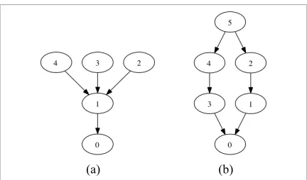
For example, in sentence (1) of figure (3), chunk 1 is clearly the argument of the verb Print

(the main predicate of the sentence), therefore there is an edge from 1 to 0 in the DG of this sen-tence as shown in figure (4a). Also, chunks 2..4 are part of the description of chunk 1, so they are the arguments of the predicate(s) describing chunk 1. This means that there must be edges from nodes 2..4 to node 1 in the DG. Similarly for sentence 2 in figure (3), chunk 5 is part of the description (hence an argument of the predicates) of chunks 2 and 4; chunks 2 and 4 are part of the description of 1 and 3 respectively; and 1 and 3 are both argu-ments of the verb Delete, the main predicate of the sentence, resulting in the DG given in figure (4b).

The following features are extracted from the DG for every sample <i,j>(1≤i<j≤n):

- Does i (or j) immediately dominate 0?

- Does i (or j) immediately dominate j (or i)?

- Does i (or j) dominate j (or i)?

- Are i,j siblings ?

- Do i,j share the same child?

Note that DG has a close relationship with the de-pendency tree of a sentence; for example, it shows the dependency relation(s) between a noun or verb and their modifier(s). Therefore it actually encodes some syntactic properties of a sentence.

7

Experiments

100 sentences from the corpus were picked at ran-dom as the development set, in order to study the relevant features and their contribution to QSD. The rest of the corpus (400 sentences) was then used to do a 5 fold cross validation. We used

SVMMulticlass _{from SVM-light toolkit (Joachims}

1999) as the classifier.

(a) (b)

Figure 4. Dependency Graphs for figure (3) sentences

1.Print [1/ every/D line/H] of [2/ the/D file/H] that starts with [3/ two/CD digits/H/S] followed by [4/ punctuation/H].

2.Delete [1/ the/D first character/H] of [2/ every/D word/H] and [3/ the/D first word/H] of [4/ every/D line/H] in [5/ the/D file/H].

Before giving the results, we define a baseline. HS03 use the most frequent label as the baseline and the similarity metric given in definition (5) to evaluate the performance. Since more than 61% of the labels in their corpus is NI, the baseline system (that leaves every sentence unscoped) has the accu-racy above 61%. In our corpus, the majority class is WS containing around 35% of the samples. NS

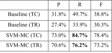
and NI each contain 34% and 31% of the samples respectively. This means that there is a slight ten-dency for having scope preference in chronological order. Therefore, the linear order of the chunks (i.e. from left to right) defines a reasonable baseline. The results of our experiments are shown in table 1. The table lists the parameters P, R, and F-score9 for our SVM-MC model vs. the baseline system. For each system, two sets of metrics have been reported: TC-based and TR-based.

Table 2 lists the sentence-level accuracy of the system. We computed two metrics for sentence-level accuracy: Acc and Acc-EZ. In calculating Acc, a sentence is considered correct if all the labels (including NI) exactly match the gold standard la-bels. However, this is an unnecessarily tough met-ric. As mentioned before (footnote 8), in practice the output of the system for the samples labeled NI

is not important; all we care is that all outscoping

(i.e. WS/NS) relations are recovered correctly. In other words, in practice, the system’s recall is the most important parameter. Regarding this fact, we define Acc-EZ as the percentage of sentences with

100% recall (ignoring the value of precision). In order to compare our system with that of HS03, we applied our model unmodified to their corpus using the same set-up, a 10-fold cross vali-dation. However, since their corpus is not anno-tated with DG, we translated our dependency features to the properties of the Penn Treebank’s phrase structure trees. Table (3) lists the accuracy

9 _{F-score is defined as F=2PR/(P+R).}

of their best model, their baseline, and our SVM-MC model. As seen in this table, their model out-performs ours. This, however, is not surprising. First, although we trained our model on their cor-pus, the feature engineering of our model was done based on our own development set. Second, since our corpus is not annotated with phrase structure trees, our model does not use any of their features that can only be extracted from phrase structure trees. It remains for future work to incorporate the features extracted from phrase structure trees (which is not already encoded in DG) and evaluate the performance of the model on either corpus.

8

Discussion

As seen in tables 1 and 2, for a first effort at full quantifier scope disambiguation, the results are promising. The constraint-based F-score of 78% is already higher than the inter-annotator agreement, which is 75% (measured using the TC-based simi-larity metric; see definition 5). Furthermore, our system outperforms the baseline, by more than 40% (judging by the constraint-based F-score). This is significant, comparing to the work of HS03, which outperforms the baseline by 16%.

We mentioned before that in our corpus in aver-age there are around 4 NPs per sentence resulting in 6 samples per sentence. Therefore the chance of predicting all the labels correctly is very slim. However, the baseline (i.e. the left to right order) does a good job and predicts the correct QSD for 27% of the sentences. At the sentence level, our model does not reach the IAA, but the performance (62%) is not much lower than the IAA (66%).

A question may arise that since the model treats

σ Baseline 61.1%

HS04 77.0%

Our Model 73.3%

Table 3. Comparison with HS04 system on their dataset

P R F

Baseline (TC) 31.8% 49.7% 38.8%

Baseline (TR) 27.4% 33.9% 30.3%

SVM-MC (TC) 73.0% 84.7% 78.4%

SVM-MC (TR) 70.6% 76.2% 73.2%

Table 1. Constraint-level results

Acc Acc-EZ

Baseline 27.0% 43.8% SVM-MC 62.3% 78.0%

the pairs of NP independently, what guarantees that the scopings are valid; that is the predicted directed graphs are in fact DAGs. For example, for a sentence with 3 NP chunks, the classifier may predict that 1>2, 2>3, and 3>1, which results in a loop! As a matter of fact, there is nothing in the model that guarantees the validness of the pre-dicted scopings. In spite of that, surprisingly all generated graphs in our tests were in fact DAGs! In order to explain this fact, we run two experi-ments. In the first experiment, corresponding to every sentence S in the corpus with n chunks, we generated a random directed graph over n nodes. Only 10% of the graphs had cycles. It means that more than 90% of randomly generated directed graphs with n nodes (where the distribution of n is its distribution in our corpus) are acyclic. In the second experiment, for every sentence with n

chunks, we created the samples <i,j> by randomly selecting values for all the features. We then tested the classifier in our original set-up, a 5-fold cross validation. In this case, only 4% of the sentences were assigned inconsistent labeling. This means that chances of having a loop in the scoping are small even when the classifier is trained on sam-ples with randomly valued features, therefore it is not surprising that a classifier trained on the actual data learns some useful structures which make the chance of assigning inconsistent labels very slim.

In general, if the classifier predicts such incon-sistent scopings, the PCFG-style algorithm of Koller et al. (2008) comes handy in order to find a valid scoping with the highest weight.

9

Summary and future work

We presented the first work on unrestricted statis-tical scope disambiguation in which all NP chunks in a sentence are considered for possible scope in-teractions. We defined the task of full scope dis-ambiguation as assigning a directed acyclic graph over n nodes to a sentence with n NP chunks. We then defined some metrics for evaluation purposes based on the two well-known concepts for DAGs: transitive closure and transitive reduction.

We use a simple model for automatic QSD. Our model treats QSD as a ternary classification task on every pair of NP chunks. A multiclass SVM together with some POS, lexical and dependency features is used to do the classification. We apply this model to a corpus of English text in the

do-main of editing plain text files, which has been annotated with full scope information. The pre-liminary results reach the F-score of 73% (based on transitive reduction metrics) at the constraint level and the accuracy of 62% at the sentence level. The system outperforms the baseline by a high margin (43% at the constraint level and 35% at the sentence level).

Our ternary SVM-based classification model is a preliminary model, used for justification of our theoretical framework. Many improvements are possible, for example, directly predicting the whole DAG as a structured output. Also, the features that we use are rather basic. There are other linguisti-cally motivated features that can be incorporated, e.g. some properties of the phrase structure trees, not already encoded in dependency graphs.

Another problem with the current system is that the extra supervision has been provided by manu-ally labeling the data (e.g. with dependency graphs). This could be done automatically by ap-plying off the shelf parsers or POS taggers, possi-bly by adapting them to our domain.

Although we consider all NPs for scope resolu-tion, scopal operators such as negation, mo-dal/logical operators have been ignored in this work. We also do not distinguish distributive vs.

collective reading of plurals in the current sys-tem.10 Incorporating scopal operators and handling distributivity vs. collectivity would be the next step in expanding this work.

Finally, since hand annotation of scope infor-mation is very challenging, applying semi-supervised or even unsemi-supervised techniques to QSD is very demanding. In fact, leveraging unla-beled data to do QSD seems quite promising. This is because domain dependent knowledge plays a critical role in scope disambiguation and this knowledge can be learned from unlabeled data us-ing unsupervised methods.

Acknowledgement

We would like to thank Derrick Higgins for pro-viding us with the HS03’s corpus. This work was supported in part by grants from the National Sci-ence Foundation (IIS-1012205) and The Office of Naval Research (N000141110417).

10 _{The corpus has already been annotated with all this}

References

Aho, A., Garey, M., Ullman, J. (1972). The Transitive Reduction of a Directed Graph. SIAM Journal on Computing 1 (2): 131–137.

Allen, J. (1995) Natural Langue Understanding, Ben-jamin-Cummings Publishing Co., Inc.

Allen, J., Dzikovska, M., Manshadi, M., Swift, M. (2007) Deep linguistic processing for spoken dia-logue systems. Proceedings of the ACL-07 Workshop on Deep Linguistic Processing, pp. 49-56.

Alshawi, H. (ed.) (1992) The core language Engine. Cambridge, MA, MIT Press.

Bos, J., S. Clark, M. Steedman, J. R. Curran, and J. Hockenmaier (2004). Wide-coverage semantic repre-sentations from a CCG parser. In Proceedings of COLING 2004, Geneva, Switzerland, pp. 1240– 1246.

Bos, J. (1996) Predicate logic unplugged. In Proc. 10th Amsterdam Colloquium, pages 133–143.

Clark P., Harrison, P. (2008) Boeing's NLP system and the challenges of semantic representation, Semantics in Text Processing. STEP 2008.

Copestake, A., Lascarides, A. and Flickinger, D. (2001)

An Algebra for Semantic Construction in Constraint-Based Grammars. ACL-01. Toulouse, France. Crammer, K., Y. Singer, N. Cristianini , J.

Shawe-taylor, B. Williamson (2001). On the Algorithmic Implementation of Multi-class SVMs, Journal of Ma-chine Learning Research.

Egg M., Koller A., and Niehren J. (2001) The constraint language for lambda structures. Journal of Logic, Language, and Information, 10:457–485.

Galen, A. and MacCartney, B. (2004). Statistical resolu-tion of scope ambiguity in Natural language. http://nlp.stanford.edu/nlkr/scoper.pdf.

Higgins, D. and Sadock, J. (2003). A machine learning approach to modeling scope preferences. Computa-tional Linguistics, 29(1).

Hurum, S. O. (1988) Handling scope ambiguities in English. In Proceeding of the second conference on Applied Natural Language Processing (ANLC '88). Koller, A., Michaela, R., Thater, S. (2008) Regular Tree

Grammars as a Formalism for Scope Underspecifi-cation. ACL-08, Columbus, USA.

Joachims, T. (1999) Making Large-Scale SVM Learning Practical. Advances in Kernel Methods - Support Vector Learning, B. Schölkopf and C. Burges and A. Smola (ed.), MIT Press.

Manshadi, M., Allen J., and Swift, M. (2009) An Effi-cient Enumeration Algorithm for Canonical Form Underspecified Semantic Representations. Proceed-ings of the 14th Conference on Formal Grammar (FG 2009), Bordeaux, France July 25-26.

Moran, D. B. (1988). Quantifier scoping in the SRI core language engine. In Proceedings of the 26th Annual Meeting of the Association for Computational Lin-guistics.

Pafel, J. (1997). Skopus und logische Struktur. Studien zum Quantorenskopus im Deutschen. PHD thesis, University of Tübingen.

Srinivasan, P., and Yates, A. (2009). Quantifier scope disambiguation using extracted pragmatic knowl-edge: Preliminary results. In Proceedings of the Con-ference on Empirical Methods in Natural Language Processing (EMNLP).

VanLehn, K. (1988) Determining the scope of English quantifiers, TR AI-TR-483, AI Lab, MIT.