Noise based Frequency Offset Modulation Simulation Model Design : For the analysis of Transmit Reference Medium Access Control in Multiple Access Ad hoc Wireless Sensor Networks

1

Faculty of Electrical Engineering,

Mathematics & Computer Science

Noise-based Frequency Offset Modulation

Simulation Model Design

For the analysis of Transmit-Reference Medium Access Control

in Multiple Access Ad-hoc Wireless Sensor Networks

Mike Kriele M.Sc. Thesis January 2018

Summary

The increasing use of wireless devices has led to more need for energy-efficient communication schemes. Recently, more effort have been put in researching low-power spread spectrum as an energy-efficient method of communication. transmitted reference (TR) is a low-power spread-spectrum technique which was introduced as a promising communication scheme used in short-range transmissions, such as wireless sensor networks. In TR modulation the transmitter sends the information signal along with the spreading signal shifted by a time or frequency offset, which can be demodulated by the receiver by applying the same offset. This simplifies the receiver architecture significantly. The receiver does thus not need to know the spreading signal used, allowing for any kind of spreading signal; including noise, giving birth to noise-based frequency-offset modulation (N-FOM).

N-FOM uses pure noise as information bearer. This is advantageous as it is easy to generate and eliminates the need for complex schemes for flattening the spectrum of the transmitted signal. Therefore, N-FOM allows for multiple-access communication by varying the frequency offset used in the receiver. However, due to the self-correlation module in the receiver, mixing terms of possible other concurrent active nodes increase the noise roughly quadratically; limiting the number of possible concurrent active links as bit error rates worsen.

Introducing a medium access control (MAC) protocol to regulate the number of concurrent transmissions could assist in overcoming this barier. Transmitted-Reference MAC (TR-MAC) is a protocol specifically designed to work with N-FOM. The protocol regulates the frequency offsets allocated to transmitting nodes and synchronized with them providing each transmitter a non-overlapping transmission opportunity to send packets. This in order to prevent collisions due to frequency offsets selected twice and to reduce too many concurrent active links. The protocol allows both transmitter-driven and receiver-driven communication. Although proven functional, TR-MAC has only been tested with abstractions of the physical layer and hard limits set on the number of concurrent active links. The creation of a new model is required that is not based on hard limits, but rather implements real physical-layer phenomena of the N-FOM physical layer. This in order to test how the physical layer

affects the medium access layer in ways that have previously not been accounted for.

Based on theTR-MAC simulation model as a starting point, the N-FOM physi-cal layer has been implemented. Physiphysi-cal layer abstractions and hard limits have been removed. A mathematical expression of the N-FOM layer has been used to model the physical layer for simulation. In order to model a more realistic channel, a Bernoulli random process has been implemented for packet error generation to determine packet error probabilities. Simulations have been performed to verify the physical layer to test its limitations and to see the effects on MAC level in a multiple-access environment.

Results show that physical layer simulation in a single-link environment is accord-ing to theory. Simulation results follow the theoretical curve on a 99.9% confidence interval. It can thus be assumed the physical layer is implemented according to the-ory. Furthermore, the limitation of the physical layer was tested. For this test, nodes were put at an equal distance and made increasingly concurrently active. It became evident the physical limit, based on the parameters set, allowed for a maximum of three concurrent active links as a maximum; thus requiring the need for a MAC pro-tocol. Multiple access simulation of the physical layer in conjunction with the MAC protocol has shown the physical layer has significant impact on the throughput of the system. The self-correlating receiver introduces mixing terms that result in a nearly quadratic increase in noise, resulting in saturation of the throughput when the num-ber of active links increases and eventually a decay due to channel contention. The resulting throughput is less than previously resulted from the TR-MAC measurement results due to these mixing terms.

Contents

Summary iii

List of acronyms vii

1 Introduction 1

1.1 Motivation . . . 1

1.2 Framework . . . 3

1.3 Goal of the assignment . . . 3

1.4 Report organization . . . 3

2 Noise-based frequency-offset modulation 5 2.1 Modulation . . . 5

2.2 Multiplexing . . . 9

2.2.1 Offset criteria . . . 10

2.2.2 Near-far effect . . . 11

2.2.3 In-band interferences . . . 11

2.3 Conclusion . . . 12

3 Transmitted reference medium access control 13 3.1 TR-MAC . . . 14

3.2 Slotted Aloha model . . . 16

3.3 TR-MAC in multiple access . . . 16

3.4 Conclusion . . . 19

4 Simulation model design 21 4.1 TR-MAC model . . . 23

4.2 Physical-layer model . . . 24

4.2.1 Modulation scheme . . . 25

4.2.2 Packet error detection . . . 26

4.2.3 Channel model . . . 29

4.2.4 Model implementation . . . 30

4.2.5 Clear Channel Assessment . . . 32

4.3 Conclusion . . . 34

5 Simulation results 35 5.1 Physical layer verification . . . 35

5.2 Peer-to-peer model testing . . . 36

5.3 Multiple access modelling . . . 38

5.3.1 Throughput performance . . . 39

5.3.2 Throughput performance with adjusted clear channel assess-ment . . . 41

5.3.3 Throughput performance comparison . . . 42

5.3.4 Throughput performance with changes in physical layer . . . . 44

5.4 Simulator efficiency . . . 45

5.5 Simulator Limitations . . . 46

5.6 Conclusion . . . 47

6 Conclusions and recommendations 49 6.1 Conclusions . . . 49

6.2 Recommendations . . . 50

List of acronyms

ACK acknowledgement

AWGN additive white Gaussian noise

BER bit error rate

CCA clear channel assessment

CI confidence interval

CNR carrier-to-noise ratio

DACS Design and Analysis of Communication Systems

EDR effective dynamic range

FSPL free-space path loss

IC integrated circuit

ICD interated circuit design

IDF integrate-and-dump filter

LO local oscillator

LOS line of sight

MA multiple access

MAC medium access control

MP multi-path

N-FOM noise-based frequency-offset modulation

NF noise figure

PN pseudo-noise

PSD power spectral density

RF radio frequency

S-Aloha Slotted Aloha

SNR signal-to-noise ratio

SS spread spectrum

TE Telecommunication Engineering

TR transmitted reference

TR-MAC Transmitted-Reference MAC

UWB ultra wideband

WALNUT Wireless Ad-hoc Links using robust Noise-based Ultra-wideband Transmission

Chapter 1

Introduction

1.1 Motivation

With the increasing use of wireless sensor devices over the past decade and an expected exponential increase of usage of such devices over the next decade [1], the need for better energy-efficient communication schemes has been imminent. Among other things this has led to more research in low-power spread-spectrum (SS) techniques [2]–[5] as an energy-efficient method of communication. SS signals are defined as low power spectral density (PSD) signals that use radio frequency (RF) signal bandwidths that greatly exceed the minimum bandwidth required to transmit their data. The signal’s spectrum is thus spread over a significantly wider RF chan-nel than needed to transmit the information signal [6], where the ratio between the transmission bandwidth and the bandwidth of the information signal is defined as the processing gain. As SS systems are mostly designed to overlay on top of other radio systems, having a large processing gain can assist in providing robustness against interference. However, receiver signal acquisition can be challenging in SS systems with large processing gains, de-spreading is not activated prior to synchronization and the received signal has to be retrieved at very low signal-to-noise ratio (SNR) levels. This is due to the fact that in SS the PSD is low and more powerful interferers are present. Additionally, in order to make SS robust against multi-path fading, com-plex receiver structures have to be used [5], [7]–[11], resulting in longer acquisition times.

In wireless sensor networks (WSNs) nodes often have strict power limitations imposed due to a limited lifetime. As the battery drains, these nodes are often con-sidered expired. The transmission and reception times of these nodes thus play an important role in their overall lifetime. As nodes are often expected to run for years (or even decades), timing plays an important role in the overall system performance of a WSN. Nodes are only allowed to wake up for short durations to transmit or re-ceive their data. Furthermore, simple and low-cost systems are often desired. In the

case of standard ultra wideband (UWB) SS transmission, it would be difficult to com-pactly design energy-efficient receivers that demodulate the received signal without knowing the spreading information used at the transmitter, yet still fulfill the demand-ing requirements set for WSNs. Complex receiver structures, e.g. rake receivers, are often required to cope with multipath effects, resulting in increased uptimes – due to slow synchronization because of finger tuning – and battery consumption; therefore significantly reducing a node’s lifetime. TR, however, could put less stress on these requirements.

Transmitted reference (TR), a slight adaption of the original SS scheme where the transmitter sends the spreading signal along with the spread information signal [12], [13], is more suitable as faster synchronization times can be achieved. An important property of TR is that complex receiver structures requiring sub-receivers to counter multipath fading, e.g. Rake receiver fingers that are tuned to a different multipath component per finger, can be omitted as the spreading signal is no longer generated in the receiver. In the case of TR the transmitter transmits a time- or frequency-shifted version of the spreading signal together with the information signal [12], [13]. This simplifies the receiver architecture to a great extent. Extracting the information signal from the spread signal requires the receiver to only know the offset used. The advantage of this approach is that the receiver does not need to generate the spreading signal used, reducing synchronization times and therefore making TR viable for low duty-cycle applications, e.g. wireless sensor devices. This also allows for noise as a reference signal, resulting in noise-based frequency-offset modulation (N-FOM). Using noise as a reference is preferable, as it is relatively easy to generate a flat additive white Gaussian noise (AWGN) spectrum and not too costly in implementation in comparison to pseudo-noise (PN) sequences or pulse positition dithering that is normally used as reference.

Furthermore, given that wireless sensor devices often operate in a WSN, multiple access (MA) is an important aspect of WSN communication. With N-FOM, having MA is easily achieved by simply adjusting the offsets used in each transmitter for different communication links. However, offsets have to be selected carefully and the possible number of simultaneous transmissions is limited, as having too many concurrent transmissions contributes to the overall noise due to cross-mixing in the receiver, leading to unacceptable bit error rates (BERs) [14]. Using an N-FOM-tailored medium access control (MAC) protocol could assist in organizing the num-ber of concurrent transmissions. Transmitted-Reference MAC (TR-MAC) [15], [16] is such protocol that has been designed as a possible suiter for TR (and N-FOM) communication.

1.2. FRAMEWORK 3

physical layer model resulting from real modelled physical layer phenomena has to be developed. This in order to evaluate the impact of N-FOM on TR-MAC as a dedicated MAC protocol in order to see if the conclusions made in [16] still hold.

1.2 Framework

This report is written for the WALNUT project as main topic of a combined master’s thesis in Computer Science and Electrical Engineering at the University of Twente. The aim of the WALNUT project is to develop new techniques for establishing robust radio links in WSNs that operate in an extremely crowded radio spectrum, at very low power, using noise-based frequency-offset TR modulation. The research encom-passes multiple topics, e.g. the N-FOM and TR-MAC schemes, currently researched and designed by PhD students within the Telecommunication Engineering (TE) and Design and Analysis of Communication Systems (DACS) research groups respec-tively. Additionally, a PhD student within the interated circuit design (ICD) group has been working on an implementation design of N-FOM on an integrated circuit (IC), but that topic is not covered as it did not fit within the scope of this thesis.

1.3 Goal of the assignment

The goal of this thesis is to investigate the behavior of TR-MAC with the N-FOM physical layer by simulating the full N-FOM system by means of a combined MAC and physical-layer model. Here the limitations of the physical layer are not given by hard limits on the number of simultaneous transmissions, but are resulting from real modelled physical layer phenomena. The result of this research should answer the following research question:

Does the full simulation model of TR-MAC and N-FOM show any effects in TR-MAC that were previously unaccounted for, which affect the performance of N-FOM as communication method for multiple-access wireless sensor net-works?

1.4 Report organization

Chapter 2

Noise-based frequency-offset

modulation

As discussed in Chapter 1, N-FOM was suggested as a more energy-efficient, and a relatively easier to implement, solution for SS communication in WSNs. However, some other limitations come with it. In this chapter a full description of N-FOM will be given to give more insight in the design criteria, its behavior and the formulas that describe it. This in order to properly model it for simulation. First, in Section 2.1, the modulation scheme is described in peer-to-peer communication, where only one transmitter is actively communicating to a receiver within a timeframe, i.e. there are no concurrent active links present. This section includes the workings of the self-correlating receiver scheme, and how frequency offsets play a role. The description of N-FOM is then extended with respect to MA communications in Section 2.2, where more insight is given in the additional design criteria for, and limitations induced by, concurrent transmissions.

2.1 Modulation

In order to determine FOM physical-layer effectiveness, extensive research on N-FOM modulation and transmission schemes has been performed by Bilalet al.[14],

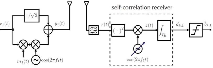
[17]–[19]. The N-FOM communication scheme shown in Figure 2.1 depicts a single-link communication. Within this scheme the spreading signal, i.e. band-limited noise, is sent along with a frequency-shifted version of the spread information signal and demodulated at the receiver by means of a known unique feature, i.e. frequency off-set. The receiver thus does not need to know the spreading signal used at the trans-mitter, but simply demodulates the received signal through self-correlation. This sig-nificantly simplifies receiver design as the spreading signal is no longer generated in the receiver for demodulation, omitting the requirement of complex receiver

Figure 2.1: N-FOM system: Modulation scheme showing a transmitter communi-cating to a receiver using an unique reference. Adapted from:[17].

tures, e.g. rake receivers, to cope with multipath effects. The whole communication scheme works as follows. At the transmitter (or user) a narrowband message signal

m1(t) is spread by the spreading signal x1(t). This signal is then shifted by using a frequency offset (f1) much smaller than the spreading signal bandwidth (Bss) [17] and is combined with the unmodulated reference signal. This modulated signal has the form

y1(t) = x1(t)

m1(t) cos(2πf1t) + 1

√

2

, (2.1)

where the 1/√2 scaling factor is chosen to make sure the information signal and spreading signal have the same mean power iny1(t). Here the frequency offsetf1is known to the receiver. A visual representation of the modulation and demodulaton process is given in Figure 2.2.

1

1

1

1 1

2.1. MODULATION 7

As can be seen the spreading signal and the data signal have significant overlap. This is due to the fact that f1 Bx, which will be explained in Section 2.2.1. The

N-FOM communication channel is initially modeled as an AWGN channel [20], [17] as a simplified representation of reality. It should be noted that this decision has been made as first-step approach to understand the workings of the N-FOM sys-tem, but that this system is actually built for a multipath environment and needs to be extended in the future. The receiver listens to the channel and receives all data, thus also noise and unwanted transmissions, transmitted over it. The received signal is then passed through a bandpass filter to (ideally) filter out all out-of-band noise. After filtering, the message of the user is retrieved by correlating the received signal

r(t) with a frequency-shifted version of itself, i.e., by selecting User 1’s frequency offset (f1 =fr) where fr is the frequency offset at the receiver. This is achieved by

squaring the received signal and applying a frequency offset by means of a local oscillator (LO) [17]. Although this might not be directly obvious from the receiver scheme depicted in Figure 2.1, when looking at Figure 2.3(a) and 2.3(b), it can be seen that first squaring a signal and then shifting in frequency equals multiplying that signal with a frequency-shifted version of itself. The reason for this is that the multiplication operation is commutative and the order in which the two consecutive operations are performed is irrelevant. The demodulated signal is then filtered using an integrate-and-dump filter (IDF). Ergo, Receiver 1 receives the bits of the Trans-mitting User 1 usingf1and any other signals present at time of reception are filtered out or considered as noise.

=

Figure 2.3: N-FOM squaring and shifting operation representations.

The performance model of peer-to-peer N-FOM is given by the BER

HereQ(x)is the Gaussian tail probability function,

Q(x) = √1

2π

Z ∞

x

exp

−u

2

2

du. (2.3)

It can be seen that the BER results from the SNR of the decision sample

SNR = 8γ

2

(25γ2₎ 1

S + 20γ+ 8S

, (2.4)

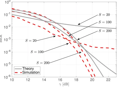
where γ = E_b/N0 is the received SNR per bit of the specific node. Eb is defined as the average received bit energy of the user and N0 is the single-sided noise PSD [17]. Furthermore, S = BxTs is the spreading factor, where Ts is the symbol

duration. From this model it can be seen that if the SNR per bit (γ) is sufficiently

large, (2.4) will reduce to the asymptote of SNRl = 8S/25. Here the SNR is not

longer dependent on the signal performance, but on the bitrate and the in-band noise.

Figure 2.4: Comparison of BER between theory and simulation, for various spread-ing factors. As taken from: [21].

2.2. MULTIPLEXING 9

is not too high, to prevent too much deviation from theoretical results, the optimal spreading factor is considered to be approximately 100 [17]. It is also apparent from Figure 2.4, that for different speading factors a different optimalγ should be selected

to reach a BER of10−3. If the SNR per bit is small, however, in-band noise will take the overhand, of which the amount of noise depends on the spreading factor.

2.2 Multiplexing

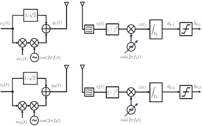
As multiple wireless sensor devices often communicate in WSNs, MA is regarded as an important aspect of WSN communication. With N-FOM having MA is easily achievable by simply adjusting the frequency offset used in a specific transmitter for different communication links, as shown in Figure 2.5. Here Receiver 1 receives data from Transmitting User 1, using frequency offset f1, and Receiver 2 received data from Transmitting User 2, using frequency offsetf2.

Figure 2.5: MA N-FOM system: Modulation scheme showing two transmitters com-municating to two receivers. Adapted from:[17].

the node of interest, is desired, self-mixing terms from other transmitters and noise products and cross-mixing terms between these and the signal of interest add to the overall contributed noise of the received signal. This results in a roughly quadratic decrease of the SNR in relation to number of users when the SNR per bit of the users are in the same order of magnitude. It can thus be observed that the squarer is the culprit of increasing the amount of noise at the receiver. However, this squaring operation is much needed for despreading the signal at the receiver, simplifying the dereferencing of the transmitted signal [22]. In the example of Figure 2.1, the number of noise products is still limited in number as only a single transmission occurs. However, when having a multitude of simultaneous transmitters present, e.g. Figure 2.5, the number of mixing terms in z(t)increases roughly quadratically; thereby also increasing noise. The overall N-FOM performance model is given by

SNRl=

8γ2

l 

 25γ

2

l + 17 N P i=1

i6=l

γ2

i + 20γl N P i=1

i6=l

γi+ 16 N−1

P i=1

i6=l N P j=i+1

j6=l

γiγj    1 S + 

20γl+ 16 N P i=1

i6=l

γi  + 8S

, (2.5)

where it is noticeable that the physical-layer behavior depends on the number of nodes in concurrent transmission, which is apparent due to the number of terms in the denominator [17]. In the case of one, two and three concurrent active links, the noise contribution increases significantly. These terms should be taken into account when modeling the physical layer in order for N-FOM to function according to Figure 2.1.

2.2.1 Offset criteria

In order for N-FOM to successfully distinguish between the reference signal and the modulated information signal, a frequency offset fi is used. This frequency offset

can be obtained by mixing one of the signals using a low-frequency LO [13]. For proper de-spreading of the signal, fi at the receiver should be chosen identical to

the offset selected at the transmitter. In order to distinguish between different trans-mitters using different frequency offsets, fi can be varied at the receiver end by

tuning the LO, allowing for MA. However, research performed by Shang et al. has

shown that the value of fi at the transmitter is not arbitrary [13], [23]. When

choos-ing a value for fi for each transmitter, one important criterion is that the selected

offsets do not cause direct interference between transmitters. Therefore it should hold that |fi−fj| 1/Tb and|fi−2fj| 1/Tb, where i 6=j, and Tb is one symbol

2.2. MULTIPLEXING 11

not distorted by the band-pass filter at the receiver [14], [18]. Additionally, in MA, a spreading factors larger than 100, i.e. the optimum spreading factor in single node communication, is desired for better SNR per bit at the receiver.

2.2.2 Near-far effect

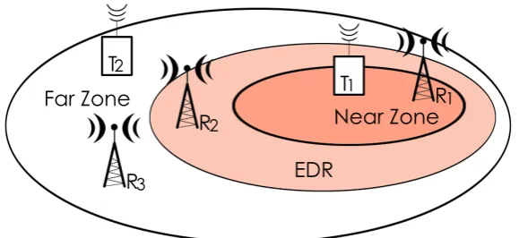
In Shang’s research the assumption was made that the signals from different users are received at the receiver with equal strengths, which is not realistic. In practice, due to the disparity in distances between transmitters, the signal from each trans-mitter experiences a different amount of attenuation. The difference between these signal strengths could lead to the near-far effect at the receiver end [17].

Generally speaking, the near-far effect (or near-far problem) occurs when the re-ceived signal power of one transmitter is significantly higher than the power rere-ceived from another transmitter, resulting in complete jamming of the signal from faraway transmitters [24], [25]. Thus, for example, when looking at Figure 2.6, in the case of receiver R1, the receiver is close to transmitter T1. Here the received power of T1 is significantly larger than the received power of T2, making it difficult (or impossible) to detect both signals and possibly jamming the weakest transmitter. This is also known as the near-problem. In case of receiver R3, transmitter T1 is too far away, resulting in the fact that T1 is too weak to be tracked by the receiver. This is called the far-problem. However, in the case of receiver R2, where the receiver remains

be-tween the near- and far boundaries, the receiver is in the so-called effective dynamic range (EDR) zone. Here both transmitters can be tracked by the receiver. The EDR is defined as the ratio between the strongest and weakest signal where the receiver can still demodulate the signals without excessive noise or distortion [24].

In research performed by Bitachon et al., it has been observed that the MA

in-terference has a significant impact on the basic N-FOM system [17]. Results have shown that the near-far problem imposes critical limitations on the N-FOM system. Here the presence of a strong user severly degradates the BER of a particular user of interest when both are transmitting simultaneously [17]. This is primarily due to the self-correlating nature of the receiver (see Section 2.1), where the decrease in performance is primarily attributed to the interference self-mixing product. Theoret-ically the limitation invoked by these self-mixing products introduced during demod-ulation result in unacceptable BERs for more than three concurrent active links [17].

2.2.3 In-band interferences

NearZone

FarZone

EDR T1

T2

R1

R2

R3

Figure 2.6:Example situation with near-far regions

For smaller bandwidths of the in-band interference, however, the signal distortion caused by the dominating term can be reduced if a frequency offset is selected that is significantly larger than the interference bandwidth [14].

2.3 Conclusion

Within this chapter a detailed literature review on N-FOM has been given. A de-scription has been made for the N-FOM physical layer in single-link communication to explain the main features of the modulation and demodulation schemes which has then been extended to performance in MA. Additional requirements for MA commu-nication have been explained and the impact of multiple concurrent active links have been described. Based on the results and conclusions of Bilal’s and Bitachon’s research, the strengths and weaknesses of N-FOM have been summarized.

Chapter 3

Transmitted reference medium

access control

As apparent from Chapter 2, the number of possible concurrent active links is severely limited as a result of the self-mixing products generated in the demodulation scheme. Invoking a restriction on the maximum number of concurrent active links allows for better BER at the receiver with proper demodulation of the desired signals. In MA wireless communication the MAC protocol is the key element in performing medium access control for the medium shared among transmitters. In general the MAC protocol regulates the network by providing addressing and channel access control mechanisms, allowing nodes to communicate within an MA network. Given that the number of concurrent transmissions has to be regulated for a proper BER at re-ception, the use of a MAC-protocol is a necessity. However, as TR (and thus also N-FOM) is designed such that the receiver receives a reference along with the in-formation signal, as opposed to coherent receivers, additional power consumption during transmission is imminent as additional signals are sent. Energy efficiency is considered an important requirement in the design of communication protocols for WSNs due to limited power [26]. Besides regulating the network in MA, the MAC layer itself has the important task to fine-tune and adapt the duty cycle of the trans-mitter and receiver in such a way that low-duty cycle communication is achievable; i.e. in order to enhance the lifetime of WSN nodes, the MAC layer should ascertain that both transmitter and receiver sleep most of the time and spend the least amount possible time to transmit, receive and listen to the channel. The MAC layer could thus exert a large amount of influence on the energy consumption, and therefore be of assistance in lowering the power consumption of N-FOM. This led to more research on a suitable energy-efficient MAC protocol, giving birth to TR-MAC.

Within this chapter, a description will be given of the design of TR-MAC and how it copes with the mechanics of the N-FOM physical layer. A description will be given on the types of communication states that occur using the TR-MAC protocol in N-FOM

communication in Section 3.1. Additionally, another model will be introduced in order to provide a better understanding on the limitations imposed by concurrent active links in N-FOM for the TR-MAC layer and how a multi-channel approach can aid in solving this issue in Section 3.2. Finally, based on the outcomes of this additional model, a full description of TR-MAC in MA will be given in Section 3.3.

3.1 TR-MAC

The main motivation for the design of TR-MAC was to exploit all the advantages of N-FOM [15], [26]–[28]. The TR-MAC protocol consists of three states, as depicted in Figure 3.1; these states are (1) first-time communication, (2) unsynchronized link, and (3) synchronized link [15].

Figure 3.1: TR-MAC communication states. As adapted from:[15].

3.1. TR-MAC 15

and shorter wake-up periods in the receivers. Subsequent to preamble reception, neighbor discovery is performed, MAC addresses are exchanged, and a link iden-tifier is determined. After initial communications, the protocol is in unsynchronized transmission. In this stage the transmitter transmits small data bursts to the receiver. If the receiver detects a packet, the transmitter is identified based on the link iden-tifier assigned. Based on this packet, receiver wake-up times are agreed upon by both ends and a unique frequency offset is allocated for communication. This allows for both receiver-driven or transmitter-driven communication. As a result, the nodes are in the synchronization stage of the protocol.

Synchronized communication is depicted in Figure 3.2(b). In this communication state, the transmitter wakes up in the agreed-upon timeslot to transmit his data along with a short preamble containing a specific frequency offset meant for a specific receiver. A receiver that wakes up and receives the short preamble directly knows whether or not the preamble is meant for it and will send out an ACK or goes back to sleep respectively. This allows for the transmitter and receiver to keep transmission to a minimum [15]. Additionaly, duty cycle adaption can be performed in order to cope with event-driven situations, to maintain energy efficiency. This makes TR-MAC a suitable TR-MAC protocol for low-data-rate applications, e.g. WSNs.

(a)

unsynchroni

zed

l

i

nk

and

f

i

rst

-t

i

me

communi

cat

i

on

(b)

synchroni

zed

l

i

nk

Preamble

with data Receive LiIdlsteen ACK ACKlisten Sleep

T

R

Overhearer x

x

T

R

Overhearer x

x t

t

t

t

t

t

Figure 3.2: TR-MAC unsynchronized and synchronized protocol. As adapted from:[15].

traffic-adaptive duty cycling and request based burst packet transfer in order to cope with increasing traffic load [16], [27]. Furthermore, multiple-link scenarios and the limitations imposed by N-FOM, e.g. the near-far effect and mixing noise products, have not been considered here.

3.2 Slotted Aloha model

In order to gain a deeper understanding of the multi-channel properties and the TR limitations imposed by N-FOM, Morshed et al. proposed a MAC-layer model

abstraction in [29] for the main purpose of providing an insight on the fundamental limitations of TR (and N-FOM) at MAC level.

For this model, single-channel Slotted Aloha (S-Aloha) was selected as a starting point [30]. Morshed et al. extended this model to a multi-channel S-Aloha version.

The model uses multiple frequency offsets implemented as seperate channels with each channel. A node can randomly and independently choose any of the channels for a time slot to transmit a packet [29]. Additionally, the model only allows for a maximum number of simultaneous transmitters, based on the system characteristics of N-FOM [17] for a successful communication.

Additionally, Morshed concluded that a larger number of available frequency off-sets yield a better thoughput in the system and thus a better efficiency with a limita-tion on the number simultaneous communicalimita-tions. Efficiency decreased when the maximum number of simultaneous communications was increased. Morshed thus found that a frequency offset based system performs best if the pool of available offsets to choose from is significantly larger than the number of allowed concur-rent simultaneous transmissions. [29] and is discussed in Section 3.3. The results gathered from the multi-channel S-Aloha model provided fundamental and deeper insight into the design criterion of a MAC protocol that exploits TR modulation.

3.3 TR-MAC in multiple access

3.3. TR-MACIN MULTIPLE ACCESS 17

this, Morshed concluded mechanisms are required that prevent simultaneous use of frequency offsets and limits the number of concurrent active links. Frequency allocation management thus had to be implemented.

Morshed concluded based on his research [16] that the available number of quency offsets is limited to 26, due to the fact that the maximum number of fre-quency offsets selected has to be much smaller than the coherence bandwidth to make sure signal and reference are affected equally by the propagation channel. This value represents the number of usable frequency offsets from a limited pool of 40 available offsets in an indoor office environment [16], which was determined by dividing the maximum value useable as frequency offset (approximately a tenth of the coherence bandwidth), by the bitrate of 25 kbps. This number is limited in order to ascertain reference and message signal are still in the same propagation chan-nel. From these offsets, one is reserved for unsynchronized transmission; hence, every node can form a maximum of 25 transmission pairs in their synchronized link state. Furthermore, the maximum available check interval duration across the net-work is divided by the maximum number of available frequency offsets, i.e., 25 time instances are allocated for node check intervals, each bound to a unique frequency offset. Results gathered from this model abstraction provided deeper insight into the design criterion of a MAC protocol that exploits TR modulation.

In the case of very dense MA networks, where an area is saturated with nodes, however, the probability of concurrent transmissions increases significantly, result-ing in more mixresult-ing products contributresult-ing to more noise in the receiver, decreasresult-ing throuhput and lowering the system’s efficiency. Due to the incorporation of channel sensing, however, this can be prevented by adding random backoff delays to nodes if the channel is sensed busy; or forcing the nodes back into unsynchronized state if too many backoff attempts have been performed and no other frequency offsets are available. Peer-to-peer communication is thus still performed to a large extent. How-ever, as the number of active links in the network increases the probability on having more concurrent active links increases as well. This is also depicted in Figure 3.3. Here Morshed plotted the thoughput against the number of active links present. As can be seen if the environment is heavily saturated by nodes, and therefore a result-ing larger number of active links, the throughput collapses as too many concurrent active links are present, resulting in too much interference at the receiver causing all concurrent communications to fail.

Figure 3.3: Throughput performance for varying number of active links. As taken from:[16].

3.4. CONCLUSION 19

protocol point of view collisions are costly. Energy is consumed by receiver and transmitter without having succesful communication, requiring retransmissions with the result that the receiver has to be awake again for reception in the future. As discussed in Sections 2.1 and 3.2, the system performance severely decreases if the number of simultaneous transmissions increases due to the unwanted mixing products. This could result in dropped packets. In other words, TR-MAC thus has to manage retransmission techniques. For the case of the unsynchronized link, trans-missions intervals are utilized to determine problems of communication. If no ACK has been received within the maximum interval duration, a problem is concluded, and retransmission has to be performed. If transmissions continue to fail for a num-ber of retransmissions, the receiver node is considered dead or out of range [16]. For synchronized transmissions, a missed ACK would mean an out-of-sync sce-nario. In order to regain synchronization, the MAC protocol has to ensure that the nodes in a synchronized pair update their transmission times or change their fre-quency offsets to prevent further collisions. The downside of this, however, is that the synchronizations are discarded too quickly if no ACK has been received. An-other solution proposed is falling back to the unsynchronized state, and attempting to regain synchronization. This has the drawback that contention increases [16].

3.4 Conclusion

Within this chapter a detailed literature review on TR-MAC has been given. A de-scription has been made of the link states of TR-MAC and how unsynchronized and synchronized link transmissions function. Additionally, it is explained how TR-MAC uses small data bursts for first-time communication instead of a preamble sampling mechanism for shorter communication times. Furthermore, an extension of TR-MAC has been given for use in MA where it exploits the TR feature of the N-FOM physical layer. Based on the results and conclusions of Morshed’s research, the strengths and weaknesses of TR-MAC have been summarized.

Chapter 4

Simulation model design

In order to test the functionality of TR-MAC, Morshed created a simulation model [16]. This simulation model has been built using the OMNeT++ [31] discrete event simulator extended with the (currently deprecated) MiXiM [32] mixed simulator pack-age, allowing for easier and more user-friendly MAC integration. Within this simula-tion Morshed implemented an abstracted version of the N-FOM physical layer char-acteristics as investigated by Bilal et al.[14], [17]–[19]. However, no mixing effects

or cross-correlation effects have been included. The transmission power has been mapped together with the carrier frequency to transmit a signal over the transmis-sion channel modelled in the TR-MAC simulation model. The channel has been characterized by Friis’s free-space path loss model, attenuating the transmitted sig-nal based on distance and carrier frequency, but omitting any fading phenomena such as shadowing and scattering effects. If the received power is larger than the receiver sensitivity, the transmission is deemed successful. Channel noise and in-terferences have thus not been taken into account [16] and a hard limit was set on the number of simultaneous transmissions. A block implementation of the MAC and physical layer in MiXiM can be seen in Figure 4.1.

In Figure 4.1 it can be seen that the TR-MAC layer is an extension of the base MAC layer of MiXiM, handling all the basic functionality of a MAC layer, e.g. upper and lower level message handling, battery access etc. This allows for modularity in the sense that different MAC layers can be applied without requiring to change a significant amount to the simulator. A similar approach applies to the base phys-ical layer. Both these layers communicate to each other through the base layer in which MiXiM handle MAC-physical layer and physical layer-MAC interaction. The MiXiM Core contains all the functions and files required to make the mixed simula-tor package run in OMNeT++. It can be seen in Figure 4.1 that Morshed extended the base physical layer with an SNR threshold decider. Within this decider block, the SNR of a signal during transmission is compared to a certain threshold. If the signal is above the threshold at all times during transmission, the communication

is deemed successful – else the packet transmission fails due to “interference” and “packet corruption”.

Simulations performed have given insight that receivers are able to synchronize with multiple transmitters allowing for better throughput. However, when the number of transmitters increases the thoughput descreases significantly, imposing a limita-tion on the number of concurrent receiver-transmitter pairs [17]. Although Morshed

et al. have proven that multi-channel TR communication using TR-MAC is functional

and successful, the physical layer is based solely on abstractions directly imple-mented in the MAC-layer. The MAC layer has not yet been simulated with a proper physical-layer implementation. A more realistic physical-layer model has to be im-plemented to test the model’s overall effectiveness.

MiXiM Core

Base Layer

Base PHY Layer

Base Decider

SNR Threshold Decider

Base MAC Layer

TR-MAC

Figure 4.1: Simulation model block diagram of MAC and abstracted physical layer implementation in MiXiM

To test TR-MAC together with the N-FOM physical layer, an integrated testing model thus had to be made. For this purpose, Bilal’s physical-layer design, dis-cussed in Chapter 2, was combined with Morshed’s TR-MAC model explained in Chapter 3. As a starting point, Morshed’s MA TR-MAC simulation model was used. The motivation to extend Morshed’s model whilst building upon deprecated software is twofold: first, the goal of this master’s thesis is to test the efficiency of the cur-rent TR-MAC model design in conjunction with a properly modelled N-FOM physical layer, not to rebuild the MAC-layer on its own; and secondly, rebuilding the TR-MAC model would take a significant amount of time, which simply does not fit within the scope of this thesis.

4.1. TR-MACMODEL 23

4.1 TR-MAC model

For the design and implementation of the TR-MAC simulation model, Morshed has used a receiver-driven communication strategy in the scope of his thesis [16]. Here the receiver allocates a frequency offset to the sender node once the first successful transmission has taken place and moves to the synchronized link state as discussed in Chapter 3 (Figure 3.1). Within this model, each node utilizes an event-based data structure in order to track events on a chronological basis. Furthermore, nodes also keep track of their neighbors and their respective communication states. Nodes are allowed to communicate to each neighbor in unsynchronized state using a dedicated frequency offset, or in synchronized state with an agreed-upon offset tracked by the receiver of interest during a prior specified timeslot. The TR-MAC model uses carrier sense and has a backoff mechanism incorporated; i.e., nodes listen to the medium prior to sending packets and back off if the channel is busy. Furthermore, a retransmission mechanism is incorporated to account for packet loss and collisions. Additionally, as discussed in [16], a maximum number of 26 frequency offsets was derived for synchronized transmission pair allocation per receiver and the over-all system parameters used for this model are given in Table 4.1, but seem rather arbitrarily chosen. The transmit power, however, is selected as twice the power of other WSN MAC-protocols as there is a 3 dB loss in the transmitter due to the sig-nal being sent twice, of which only half contains the information. This assumption, although seems logical, does not completely hold as there is an additional 7.8 dB loss in SNR due to the noise-mixing products in the self-correlation receiver in the optimal case, resulting in a total of at least 10.8 dB deficiency in comparison to other systems.

Table 4.1: TR-MAC system parameter values. As derived from: [16].

Preamble duration Header duration Data duration ACK duration Periodic listen duration Tx power Rx power Sleep power

8 bits 16 bits 32 bits 24 bits 40 bits 2 mW 1 mW 15 µW

Whenever a node initializes and passes the INITIALIZATION state for the first time, the respective node goes toSLEEPand starts in the unsynchronized link state. Within this SLEEP phase the node uses predetermined wakeup times to sense the medium for activity of other nodes using the standardized frequency offset and moves to the CLEAR CHANNEL ASSESSMENT state. If nothing is received and the node has no packets to send, it returns to the SLEEPstate and schedules a new wake-up time after a globally known check-interval duration to prevent possible channel con-tention. If any communication was detected during the CLEAR CHANNEL ASSESSMENT state, the node moves to theWAIT DATA state until a complete preamble data packet is received. If the data is not of interest for this specific node, or if an ACK is re-ceived, the preamble is discarded and goes back to itsSLEEPstate. However, if the received preamble packet is destined for the node, the node moves to theSEND ACK state to send an ACK back to the respective sender.

Within the SEND ACK state, a node can decide to move to the synchronized link state if the transmitting node is willing to synchronize and a shift is made to the syn-chronized state for receiver-driven communication. Furthermore, nodes are added to a neighbor list with agreed-upon frequency offset and wake-up time for commu-nication if they were not in there yet. Additionally, this synchronized listen event is added to the event list. In this SEND ACKstate, the current node sends an ACK back to the transmitting neighbor node and returns to itsSLEEPstate. Whenever this node wakes up in its next periodic wake-up periods, the node can either listen using the standardized frequency offsets for detecting or sending to unsynchronized links; or the node can wake up during an agreed time instance to receive or send a packet from or to a known synchronized neighbor pair using a predetermined frequency offset. This, however, depends on which event is scheduled first.

In the case an ACK is missed, the respective node schedules a retransmission event in the event list specifying the receiving node of interest. If there are multi-ple failed retransmission attempts, i.e., no ACKs received; the transmitting node will move back to the unsynchronized state and drop the packet after a maximum num-ber of retransmissions. Additionally, a random backoff period is introduced between retransmissions in the unsynchronized state to prevent channel contention.

4.2 Physical-layer model

4.2. PHYSICAL-LAYER MODEL 25

Figure 4.2: TR-MAC model operation finite state diagram. As taken from:[16].

4.2.1 Modulation scheme

modeling changes on bit-level where every step in the N-FOM modulation scheme that alters the signal is discribed and accounted for into OMNeT++ would require a large number of relatively complex calculations per transmission, significantly slow-ing down the simulator. In order to overcome this issue, Bitachon’s N-FOM node SNR mathematical expression [17] that describes the BER as a function of the re-ceived SNR per bit, as explained in (2.5) in Section 2.2, has been used as a starting point to model the N-FOM modulation scheme. It should, however, be noted that the calculated node BER through the SNR at the receiver (SNRl) is the SNR after

de-modulation and the IDF, and therefore should not be confused with the SNR directly at the antenna of the receiver where it is usually measured. This is advantageous for this specific use-case as the SNRl closed-form expression completely

incorpo-rates the modulation and demodulation effects; consequently describing the N-FOM physical-layer behavior through a black-box principle. Resulting from (2.5) the BER can be calculated by (2.2) as explained in Section 2.1.

The use of (2.5) for modeling the N-FOM physical layer behavior is justifiable as Bilal et al. have proven that the theoretical closed-form approximation roughly

follows simulations from the full N-FOM communication model for large values of the spreading factor [21]. The theoretical closed-form expression roughly follows the results from simulation down to approximately 10−3 BER. This is good enough for N-FOM simulation purposes as is expected that signals below 10−3 BER have a significantly small packet error probability; i.e. packets have a chance on packet errors in the range of 1 percent or less, with appriopriate spreading factor chosen, resulting in practically no errors after demodulation. Additionally, it should be noted that the objective of this thesis is to test TR-MAC using the N-FOM physical layer; not to verify it, as this has already been done in Bilal’s research.

4.2.2 Packet error detection

con-4.2. PHYSICAL-LAYER MODEL 27

current active links in the network are detected; the latter was modeled in the MAC layer as an abstraction. Additionally the physical layer abstraction used was a sim-ple peer-to-peer communication model provided by the base physical layer and SNR threshold decider blocks as depicted in Figure 4.1. Here the SNR was described as the carrier-to-noise ratio (CNR):

CNR= Pr

Pn

= Pt/LFSPL

N0Bss

= Pt

λ

4πd

2

kTsysBss

(4.1)

where Pr is the received power at the antenna, Pn the in-band noise power, Pt the transmitted power, LFSPL the free-space path loss, λ the wavelength of the trans-mitted signal, d the distance between transmitter and receiver, and N0 the thermal noise PSD which is given by Boltzmann’s constant k and the system temperature Tsys in Kelvin. The system temperature is descibes as

Tsys =Ts+Te =Ts+ (Fs−1)T0, (4.2)

whereTs is the antenna temperature,Te the equivalent temperature of the receiver,

Fs the standard noise figure (NF), and T0 room temperature. Often it is considered that Ts = T0, which is practical in case the antenna sees a lot of objects in its field of view that are room tempeature (T0). This was also considered in Morshed’s abstraction, resulting in

Tsys =FsT0. (4.3)

Evidently, it thus follows that

CNR= Pt

λ

4πd

2

kT0FsBss

(4.4)

It should, however, be noted that this does not describe any cross-mixing effects due to the N-FOM self-correlation demodulation scheme.

For the case of the N-FOM physical-layer model, instead of a static threshold a stochastic process is chosen where the packet error generation is determined by a random process to model a channel that is not 100 percent reliable. In N-FOM additional noise products are generated as a result of cross-mixing. The amount of noise at the receiver highly depends on the number of concurrent active links present in the transmissions period of the node of interest. The received SNR (SNRl) after

demodulation is thus primarily determined by the active links’ SNR per bit. Based on the SNRla BER can be calculated. The acceptence of a packet is then characterized

n2 n1

Figure 4.3: Two packet transmissions by separate transmitters with partially over-lapping packets.

process is a Bernoulli process with success probability 1−p, where p ∈ [0,1] is the packet loss probability [33]. Within this process it is assumed bit errors occur independent of each other. Therefore the packet loss probability can be calculated as:

p= 1−(1−BER)n, (4.5)

where theBER is calculated using (2.2) andn is the packet length in bits. Here the

packet is assumed to be lost if p is larger than a randomly selected and uniformly

distributed value between 0 and 1.

It should, however, be noted that (4.5) only holds if concurrent transmissions are perfectly synchronized. In the case of not exactly overlapping transmissions for concurrent active links, the packet loss probability changes as the BER changes when more packets starts overlapping. This is shown in Figure 4.3. Here it can be seen that during packet transmissions of Tx1 the packets are partially overlapping the transmitting packets of Tx2. Here the first n1 bits of packets from Tx1 do not overlap with Tx2, resulting in a different BER than the following n2 bits. The correct packet loss probability function would then be

p= 1−(1−pb,1)n1(1−pb,2)n2. (4.6)

4.2. PHYSICAL-LAYER MODEL 29

p= 1−

N

Y

i=1

(1−pb,i)ni, (4.7)

where N is the total number of different overlaps, and thus different BER values,

within a single packet transmission.

4.2.3 Channel model

In order to have a fully functioning physical layer model, the propagation channel between receiver and transmitter has to be described. For the current channel model Friis’s free space path loss model has been used resulting in the following free-space path loss (FSPL):

L= 4πd λ 2 , (4.8)

where λ is the wavelength corresponding to the carrier frequency and d is the

dis-tance between transmitter and receiver. Effects such as shadowing and small-scale fading thus have not been included. The primary reason for this is that (2.5) also does not account for these effects. Using a fading model in combination with (2.5) would give incorrect results. This, because in (2.5) the assumption has been made thatγl is a known value, whereas in the case of fading γl varies and has delay

dis-persion effects. These effects have not been accounted for in (2.5) as it is assumed during derivation of the equation that the received signal is a scaled representation of the transmitted signal without distorted. The main motivation for not updating (2.5) is that the scope of this thesis is to design a simulation model incorperating both N-FOM and TR-MAC from Bilal’s and Morshed’s research respectively. As not enough research has been performed to generate a closed-form approxation of the N-FOM physical layer that includes fading, it simply does not fit within the scope of this thesis.

However, as explained in Section 4.1, Morshed et al. defined the maximum

number of available useable frequency offsets roughly based on an indoor office environment. The Friis’s free-space path loss model, however, does not take this indoor office environment into account as it is defined for free space and therefore has a different path-loss exponent. Extending Friis’s free-space path loss model to the log-distance pathloss allows for the use of different path loss exponents and is given by

LdB = PL (d0) + 10αlog10

d d0

In (4.9), αis the path-loss exponent and dis the distance. PL (d0) is defined as the free-space path loss at reference distance d0, which in short-range systems, such as N-FOM in an office environment, is approximately 1 m [34]. This results in

LdB = 20 log10

λ

4π

+ 10αlog₁₀(d), (4.10)

which equals to

L= 4πd (α

2)

λ

!2

. (4.11)

Here it is assumed that communication is done on a single floor and no walls or floors/ceilings are penetrated between transmitter and receiver, i.e. there are no wall absorption losses. As it is an office environment, the path-loss exponent is assumed to be approximatelyα= 3.3[35]–[37].

4.2.4 Model implementation

The N-FOM physical layer is implemented in OMNeT++ and MiXiM as an extention to the base physical layer, as depicted in Figure 4.1, as follows. From the base physical layer a transmission powerPxis selected at the start of the simulation. This

signal is sent through the FSPL channel and received as:

Pr =

Px

L . (4.12)

Based on this an SNR per bit (γ) has to be generated. However as TR-MAC and

N-FOM are built as modules in the MiXiM package, they are required to extend MiXiM’s basic functions in order to maintain the ability to interchange physical layers and MAC-layers. To calculate the SNR per bit, an extension has thus been written on top of MiXiM’s basic physical layer and thereby extending MiXiM’s basic SNR function which actually provides the CNR of a transmitting node directly after reception. This CNR is calculated as

CNR = Pr

Pn

= Px/L

N0Bss

, (4.13)

whereasγ is defined as

γ = Eb

N0

4.2. PHYSICAL-LAYER MODEL 31

In order to calculate the SNR per bit (γ) based of MiXiM’s standard CNR function a

conversion has to be made. SinceEb =PrTbis the received bit energy, where Tb is the bit transmission time, it can be solved that

CNR = Pr

N0Bss

= PrTb

N0BssTb

= Eb

N0B_Rss b

= γ

S, (4.15)

where Rb is the bitrate and S is the spreading factor. In other words, γ can be obtained by multiplying the SNR calculated through MiXiM by the spreading fac-tor. This calculation is performed for each concurrent active link present during the transmission period of the desired node. Based on the SNRs per bit calculated for each concurrent transmitter and selecting an appropriate spreading factor (S),

SNRlis calculated using (2.5). Depending on the number of concurrent active links,

extra conditions apply for the summations performed in the denominator, adding additional noise (cross-)products. This SNRl function thus describes the SNR per

bit after demodulation and mixing. Using SNRl the BER is calculated and checked

using the packet error probability function (4.7) as described in Section 4.2.2, to determine whether or not the packet is lost due to bit errors induced during packet transmissions. This results in a different simulation model block diagram than shown in Figure 4.1, an updated version of the simulation model block diagram is depicted in Figure 4.4.

MiXiM Core

Base Layer

Base PHY Layer

Base Decider N-FOM PHY

TRDecider

Base MAC Layer

TR-MAC

Figure 4.4: Simulation model block diagram of MAC and N-FOM physical layer im-plementation in MiXiM

within the scope of this thesis, simulations performed will primarily cover N-FOM and TR-MAC interaction scenarios for as well peer-to-peer as MA communications.

4.2.5 Clear Channel Assessment

As explained in Section 4.1 nodes will move to the SLEEP state for a random dura-tion if any communicadura-tion was detected during theCLEAR CHANNEL ASSESSMENTstate. Originally in Morshed’s design this occured at any form of activity in the channel, re-sulting in the fact that only a single transmitter is allowed to transmit transmit at a specific transmission opportunity; blocking out the possibility of concurrent trans-missions. However, in the case of N-FOM, a signal can still properly be received if concurrent active links are present, as every transmitter has a unique frequency off-set. This, given the signals of these transmitters are sufficiently weak enough with respect to the transmission of interest. In order to determine the influence of the mixing products introduced by (2.5), the CLEAR CHANNEL ASSESSMENT state thus has to be altered. In order to do so a threshold has been implemented in the physical layer, where nodes in the CLEAR CHANNEL ASSESSMENT state check if the SNR of the signal in the channel received is below a specific value. This threshold is based on theoretical analysis on how the SNR per bit of a specific transmitter influences the BER of the received signal of the node of interest. This is depicted in Figure 4.5.

4.2. PHYSICAL-LAYER MODEL 33

In the scenario of Figure 4.5 it is considered that there is a receiver simultane-ously listening to two transmitting users using different frequency offsets. In this case the SNR per bit of User 2 (γ2) is fixed for different values and the BER of both users is plotted as a function of the SNR per bit of User 1 (γ1). Here, User 1 is the node of interest and User 2 is an interfering node. It is evident that the BER of User 2 deteriorates when the SNR per bit of User 1 increases, improving the BER of User 1. Mathematically, this relation can be defined as

BER =Q√SNR, SNR = 8γ

2 1 (25γ2

1 + 17γ22+ 20γ1γ2)/S+ (20γ1+ 16γ2) + 8S

,

(4.16) where the SNR in (4.16) is a simplification of (2.5). Given that a proper signal re-ception for User 1 is desired – as a general rule of thumb this means a BER lower than10−3 – whereas the signal of User 2 is desired to have the least amount of in-fluence as possible – i.e. a BER higher than10−3, a maximum SNR per bit of User 2 can be defined for which signal reception of User 1 can be assumed to be received correctly a significant amount of the time. In Figure 4.5, cross-sections are indicated and compared to the theoretical BER requirement. Here it is evident that in order to have an acceptable BER for User 1, while having little influence of User 2, the SNR per bit of User 2 should be lower than 20 dB. This, assuming that the SNR of User 1 is not too weak to begin with, which is mostly not the case unless very large distances are covered. In other words

γ2 ≤20 dB. (4.17)

This generalisation does not only hold for 2 concurrent transmitters. Based on Cauchy-Schwarz inequality it can be stated that if the mixing products of n amount of concurrent transmitters that are not of interest with a total SNR per bit of 20 dB has equal or less impact on the BER of User 1 than a single concurrent active transmitter’s SNR per bit of 20 dB. It thus should hold that

γmixingprod≤γ2 ≤20 dB, (4.18)

given that the noise products of (2.5) are equal to the noise products of (4.16) with aγ2 of 20 dB for a specific value ofγ1, i.e.

    17 N X i=1

i6=l

γ2i + 20γl=1

N X i=1

i6=l

γi+ 16 N−1

X i=1

i6=l N X j=i+1

j6=l

γiγj    

1

S + 16

N X i=1

i6=l

γi= 2000γl=1+ 17·104

1

S + 1600.

Simply said, if the channel is sensed and the SNR per bit of the signal directly at the antenna is lower than 20 dB, the physical layer will tell the MAC layer it can move to the SEND DATA state, else it will back off randomly and move to the SLEEP state. It should, however, be stated that this threshold method does not ac-count for possible near-far effects between transmitters and receivers during the CLEAR CHANNEL ASSESSMENT state, it could thus occur that a receiver is placed in such a way that the transmitter of interest will not transmit due to a too strong signal present whereas it would’ve been acceptible due to the near-far effect if the other transmitter is further away from the receiver – or vice-versa.

4.3 Conclusion

Chapter 5

Simulation results

5.1 Physical layer verification

As discussed in Chapter 2, a large limitation on the physical-layer side is that if the number of concurrent active links increases the received signal BER also increases significantly due to additional noise and mixing terms generated during demodula-tion. In order to verify this phenomenon and to get an idea on the maximum number of active concurrent links allowed before the BER reaches unacceptible values and the received signal is saturated with noise, an initial test has been performed. For this test the physical layer as modelled by (2.5) and the channel as defined in (4.10) have been used. The MAC layer has been omitted, to prevent any regulation on communication of nodes in the network; resulting in all nodes trying to communicate at the same time.

In this simulation a single node is selected to be a receiver and an increasing number of transmitting nodes, using unique frequency offsets, are added step-by-step. For the transmitting nodes, distances are selected to be equal in respect to the receiving node, with line of sight (LOS) communication. Furthermore, the distance is selected such, that in peer-to-peer communication theSNRl reaches its equilibrium

state as discussed in Section 2.1, with as results the packet error probability is very small without mixing products of interfering nodes. This to ensure packets only have interference from mixing products from other active nodes. Distances for transmitting nodes to receiver have been chosen equal, so no near-far effect is present. Other variables are chosen such that it is according to Table 4.1 and a spreading factor of 200 has been chosen. In order to generate results, N-FOM is simulated using the MiXiM package, as discussed in Chapter 4, to generate and transmit 2000 packets at each transmitter. From this simulation the total number of dropped packets due to interference, i.e. mixing products, is divided by the total number of transmitted packets to give a percentage of accepted and dropped packets for a specific number of concurrent active transmitters. Results are given in Figure 5.1.

Figure 5.1: Packet acceptance in “physical layer only” interaction with increasing number of concurrent active links, where d= 3m,α = 3.3, Pt = 2mW,

andS = 200.

As apparent from Figure 5.1, the percentage of dropped packets significantly increases with more than two concurrent active links simultaneously trying to com-municate to the same node; at least 90% of the packets drop due to interfering nodes. At four or more concurrent active links the mixing noise products are pre-dominantly present and all information is lost. As the concept of N-FOM is to use it in an MA environment, it is expected that more nodes will be present than the four only tested so far. It is thus clear the mixing products severely limit the performance of N-FOM without proper medium access control. It should thus be made sure that at all times a maximum of two nodes are concurrently active in order to maintain a proper packet acceptance rate. Morshed’s TR-MAC design should do just this, but needs to be validated with N-FOM as discussed in Chapter 3 and Chapter 4. However, first it should be verified that the stochastic validation process discussed in Section 4.2.2 is implemented correctly. This is discussed in Section 5.2.

5.2 Peer-to-peer model testing

5.2. PEER-TO-PEER MODEL TESTING 37

cross-mixing of concurrent active links is not always present. It is therefore important to ascertain that the N-FOM physical layer simulation model is working correctly in conjunction with TR-MAC in single transmitter-receiver communication and the vali-dation process used has outcomes that do not deviate too much from the theoretical values.

For the peer-to-peer simulation a single node is selected as receiver and a single transmitter is set at predetermined distances in LOS from the receiving node, such that the theoretical packet error probabilities are 0, 30, 50, 70, and 100 percent respectively. Futhermore, receiver sensitivy limitations are disabled in order to make sure only the possible deviation of the transmission success process described in Section 4.2.2 is measured. Other variables are again chosen such that it confers with Table 4.1, with a spreading factor of 200, a pathloss exponent of 3.3 and the physical layer modeled as discussed in Chapter 4, to generate and transmit 4000 packets at the transmitter. Within this simulation, the number of dropped packets at the receiver is divided by the total number of packets received to calculate the percentage of failed packets. Results are given in Figure 5.2(a) and Figure 5.2(b).

In Figure 5.2(a) the percentual packet error pobability is given with 99.9% confidence interval (CI). The confidence interval was calculated as

¯

X±z∗√σ

n, (5.1)

where_X¯ _{is the sample mean,σis the sample standard deviation,nthe sample size,} andz∗ the z-value. Here the sample mean is calculated as

¯

X = 1

n

N

X

i=1

Xi, (5.2)

and the standard deviation as

σ = v u u t 1

n−1

N

X

i=1

Xi−X¯

2

. (5.3)

and calculated, as it is still an approximation. However, it can be stated that the deviations observed are not significant enough to assume the transmission success process used is invalid.

Figure 5.2(b) depicts the packet error probability on a logarithmic scale. Here it can be observed that the packet error probability simulation plot (and its deviations) closely follows the curve of the BER plotted against the SNR per bit in [17]. This acts as an alternative presentation in percentages for better overview in probabilities. Hence, it can be concluded that the N-FOM physical layer is implemented properly enough in the simulator, allowing for further and more extensive testing of N-FOM on the TR-MAC-layer.

(a) percentual packet error probability with 99.9% CI

(b) logarithmic packet error probability with 99.9% CI

Figure 5.2: Package error probability plotted against SNR per bit at a 99.9% CI from simulation in respect to theory, whereα= 3.3, P_t = 2mW, andS = 200.

5.3 Multiple access modelling