Abstract— In a previous study, we proposed a novel method for approximating multi-dimensional time-series, called multi-dimensional time-series Approximation with use of Local features at Thinned-out Keypoints (A-LTK), which was shown to obtain a sufficiently accurate value when reduced storage cost is a requirement. In this study, we propose a modified version of this method where two changes are made to address the problem of degraded accuracy caused by high dimensionality. Our evaluation indicates that the Modified A-LTK is capable of achieving similar or superior accuracy compared with A-LTK and other existing methods but with the added advantage of reduced processing costs.
Index Terms—multi-dimensions, times series, classification, approximation, modified A-LTK
I. INTRODUCTION
APID progress in the development of sensor devices has resulted in sensors with the ability to continuously acquire multiple time series data. For example, motion capture systems can output multiple streams of observed stream data on each marker position [5]. The latest smartphones and tablets can measure geographical locations which means that data from multiple sensors equipped with mobile devices can be used for activity estimations. Sensors are also useful for predicting extreme weather, for example, some parts of the world are repeatedly struck and damaged by heavy storms such as hurricanes, typhoons, or cyclones.
Because predicting the track of a storm is important for preventing damage, data of the characteristics for storms is measured on a continuous basis [6]. The data, which is generated as multi-dimensional time-series, includes the location, speed, direction, max-wind-velocity, low-atmospheric-pressure, force-win-radius of the storm.
Many methods have been proposed for modeling and classifying multi-dimensional time-series data, but these methods lead to a problematic relationship between cost and accuracy. In our previous study, we proposed a novel method for approximating multi-dimensional time-series, called multi-dimensional time-series Approximation with use of
Yu Fang is a student of Graduate School of Information Science and Engineering, Ritsumeikan University, Kusatsu, Shiga, JAPAN.
(corresponding author, e-mail: [email protected]).
Hung-Hsuan Huang is an associate professor of Graduate School of Information Science and Engineering, Ritsumeikan University, Kusatsu, Shiga, JAPAN. (e-mail: [email protected]).
Kyoji Kawagoe is a professor of Graduate School of Information Science and Engineering, Ritsumeikan University, Kusatsu, Shiga, JAPAN. (e-mail:
local features at thinned-out keypoints (A-LTK) [1], which obtains a sufficiently accurate value when reduced storage cost is a requirement. In this study, we propose a modified version of A-LTK in terms of which are similarity value normalization and a modification of the similarity definition, which address the crucial problem of degraded caused by high dimensionality.
II. MULTI-DIMENSIONAL TIME SERIES CLASSIFICATIONS AND A-LTK[1]
As is known, a multi-dimensional time-series is defined as a sequence of vectors, that is, TS = <v1, v2, ..., vn>, where vk is a d-dimensional vector at a time tk. When k=1, TS is a time series of scalar values, that is one dimensional time series. For our purpose, the assumption is made that the length of TS, n, is a variable. A query Q is also defined as a sequence of d-dimensional vectors qk. Q=<q1, q2, ..., qm>.
Many methods that use multi-dimensional time-series for classifications, searching, and clustering, have been proposed to date. However these methods lead to a problematic relationship between cost and accuracy. We have proposed a novel method for approximating multi-dimensional time-series, named multi-dimensional time-series Approximation with use of Local features at Thinned-out Keypoints (A-LTK).
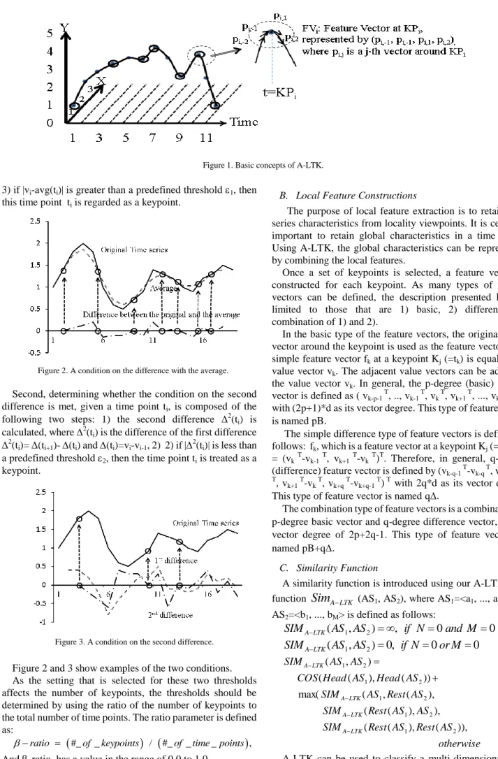
There are two important concepts with A-LTK: 1) thinned-out keypoints and 2) local feature construction. The basic concepts are illustrated in Figure 1. First, only those time points which are necessary for representing multi-dimensional time-series are selected and used as time-series approximation. The remaining time points are those around which local features are constructed and named keypoints. No features are constructed at the removed time points what were removed.
A. Thinned-out Keypoints
The purpose of thinned-out keypoints is to represent an original multi-dimensional time series using vectors that are as small as possible. Extraction of a smaller number of keypoints can reduce the computational cost to calculate a dynamic programming scheme such as that used in DTW or LCS.
Two types of thinned-out conditions are introduced to select keypoints, namely, a condition on difference with the average and a condition on the second difference.
First, determining whether the condition on the difference with the average is met, given a time point ti, is composed of the following three steps: 1) the average vector avg(ti) is calculated, 2) the difference between vi and avg(ti) is checked,
Modified A-LTK: Improvement of a
Multi-dimensional Time Series Classification Method
Yu Fang, Hung-Hsuan Huang, and Kyoji Kawagoe
R
3) if |vi-avg(ti)| is greater than a predefined threshold 1, then this time point ti is regarded as a keypoint.
Second, determining whether the condition on the second difference is met, given a time point ti, is composed of the following two steps: 1) the second difference 2(ti) is calculated, where 2(ti) is the difference of the first difference
2(ti)= (ti+1)- (ti) and (ti)=vi-vi-1, 2) 2) if |2(ti)| is less than a predefined threshold 2, then the time point ti is treated as a keypoint.
Figure 2 and 3 show examples of the two conditions.
As the setting that is selected for these two thresholds affects the number of keypoints, the thresholds should be determined by using the ratio of the number of keypoints to the total number of time points. The ratio parameter is defined as:
#_ _ / #_ _ _ ,
ratio of keypoints of time points
And -ratio has a value in the range of 0.0 to 1.0.
B. Local Feature Constructions
The purpose of local feature extraction is to retain time series characteristics from locality viewpoints. It is certainly important to retain global characteristics in a time series.
Using A-LTK, the global characteristics can be represented by combining the local features.
Once a set of keypoints is selected, a feature vector is constructed for each keypoint. As many types of feature vectors can be defined, the description presented here is limited to those that are 1) basic, 2) difference, 3) combination of 1) and 2).
In the basic type of the feature vectors, the original value vector around the keypoint is used as the feature vector. The simple feature vector fk at a keypoint Kj (=tk) is equal to the value vector vk. The adjacent value vectors can be added to the value vector vk. In general, the p-degree (basic) feature vector is defined as ( vk-p-1 T, .., vk-1 T, vk T, vk+1 T, ..., vk+p-1 T) T with (2p+1)*d as its vector degree. This type of feature vector is named pB.
The simple difference type of feature vectors is defined as follows: fk, which is a feature vector at a keypoint Kj (=tk) is fk
= (vk T-vk-1 T, vk+1 T-vk T)T. Therefore, in general, q-degree (difference) feature vector is defined by (vk-q-1 T-vk-q T, vk T-vk-1
T, vk+1 T-vk T, vk+q T-vk+q-1 T) T with 2q*d as its vector degree.
This type of feature vector is named q.
The combination type of feature vectors is a combination of p-degree basic vector and q-degree difference vector, with a vector degree of 2p+2q-1. This type of feature vectors is named pB+q.
C. Similarity Function
A similarity function is introduced using our A-LTK. The function
Sim
A LTK (AS1, AS2), where AS1=<a1, ..., aN> and AS2=<b1, ..., bM> is defined as follows:0 0
, ) ,
( 1 2
AS AS if N and M
SIMALTK
0 0
, 0 ) ,
(
1 2
AS AS if N or M
SIM
A LTKotherwise AS Rest AS Rest SIM
AS AS Rest SIM
AS Rest AS SIM
AS Head AS
Head COS
AS AS SIM
LTK A
LTK A
LTK A LTK A
)), ( ), ( (
), ), ( (
), ( , ( max(
)) ( ), ( (
) , (
2 1
2 1
2 1
2 1
2 1
A-LTK can be used to classify a multi-dimensional time series using the above similarity function. The preliminary Figure 1. Basic concepts of A-LTK.
Figure 2. A condition on the difference with the average.
Figure 3. A condition on the second difference.
experiments, in which we focused on two-dimensional time series, supported to conclude that our method was capable of attaining similar or superior accuracy compared with other existing methods with the additional advantage of a smaller processing cost.
D. Existing Problem
When we conducted experiments with A-LTK using three-dimensional or higher dimensional time-series data, we found the results obtained were not as satisfactory as we expected. We found that this was attributable to the high length of the data when high dimensional time-series were used. The similarity function was defined as a loop that accumulated the value of the cosine, where the value of
A LTK
Sim
became higher when the two time series were more similar. Thus, due to the high differences in the lengths of the data, the most similar data were the longest.We consider three time series, i.e., (1), (2), and (3), as shown in Figure 4. These are all two dimensional time series, i.e., sequences of two-dimensional vectors of X and Y.
Intuitively, time series (2) is more similar to time series (3), rather than time series (1). However, it is possible that the value of
Sim
A LTK ((1), (2)) is greater than that ofA LTK
Sim
((2), (3)). For example, according to the definition used by A-LTK, the similarity value is a sum of the individual similarities of the most similar pairs. This similarity is defined using the cosine function. In this example, the vector directions may be close for a pair at a certain time-point in (1) and (2), where the similarity is maximized. Thus, series (2) may be considered to be more similar to (1) at this point. To solve this problem, we propose a modified method (Modified A-LTK), which is described in detail in the next section.III. MODIFIED A-LTK
To address the problem of degraded accuracy, we propose a version of the A-LTK method with two modifications:
similarity value normalization and modification of the similarity definition.
A. Modified A-LTK (a) : similarity value normalization As the first modification, we introduce the normalization of similarity values by calculating
Sim
A LTK . The new similarity functionSim
A LTK (AS1, AS2), where AS1=<a1, ..., aN> and AS2=<b1, ..., bM> is defined as follows:1 2
( , ) , 0 0
A LTK
SIM
AS AS if N and M
1 2
( , ) 0, 0 0
A LTK
SIM
AS AS if N or M
1 2
1 2
1 2
1 2
1 2
( , )
( ( ), ( ))
max( ( , ( ),
( ( ), ),
( ( ), ( )) / 1 ,
A LTK
A LTK A LTK A LTK
SIM AS AS
COS Head AS Head AS
SIM AS Rest AS
SIM Rest AS AS
SIM Rest AS Rest AS
otherwise
where we divide
Sim
A LTK by (M+N-1).This modification make the influence on the results be less when the number of matched pairs is high, which occurs frequently in high dimensional time series.B. Modified A-LTK (b): modification of the similarity definition
As the second modification, we calculate the Euclidean distance between feature vectors instead of the cosine similarity. The definition of
Sim
A LTK (AS1, AS2), where AS1=<a1, ..., aN> and AS2=<b1, ..., bM> is as follows:1 2
1 2
( , ) 0, 0 0
( , ) , 0 0
A LTK A LTK
SIM AS AS if N and M
SIM AS AS if N or M
1 2
1 2
1 2
1 2
1 2
( , )
( ( ), ( ))
min( ( , ( ),
( ( ), ),
( ( ), ( )),
A LTK
A LTK A LTK A LTK
SIM AS AS
Dis Head AS Head AS SIM AS Rest AS
SIM Rest AS AS SIM Rest AS Rest AS
otherwise
Thus, two series are more similar when the value of
A LTK
Sim
is smaller. Therefore, a pair of dissimilar data in two time-series will not be considered similar and they will not be matched.IV. Evaluations A. Test Data Sets
We used two datasets in our experiment: the Mouse-Dataset and the Action-Data.
The Mouse-Dataset comprises two-dimensional data, which are sketches of simple pictures, that belong to four categories: circles, squares, triangles, and waves. The number of data items in each category is 20.
The Action-Dataset comprises three-dimensional trajectory data, which were collected by obtaining trajectory data from four different actions performed by parts of people’s bodies. The trajectories were captured and outputted using a Kinect sensor. Each action comprises three or five trajectories of different lengths.
In these experiments, we focused on multi-dimensional time series, where we compared the Modified A-LTK with A-LTK and dynamic time warping (DTW).
B. Experiments
The following four experiments were conducted: Modified A-LTK(a) accuracy with two-dimensional data (EX1), Modified A-LTK (a) accuracy with three-dimensional data Figure 4. Image of Data Length Difference
X Y
(EX2), Modified A-LTK(b) processing time (EX3T) and Modified A-LTK(b) accuracy (EX3A). The Mouse Dataset was used for EX1, while the Action- Dataset was used for EX2,EX3A and EX3T. The 1-NN classification task, which is a basic and simple application of time series for comparison, will be considered to evaluate the accuracy in this section.
EX1: In this experiment, classification by the Modified A-LTK(a) was tested in terms of its accuracy using the Mouse-Dataset. The accuracy was defined as: (Number of successful classifications) / (Number of classification trials).
The number of trials was equal to the number of the test data set, i.e., 80. The accuracy of the Modified A-LTK(a) was compared with that of A-LTK.
EX2: In this experiment, classification by the Modified A-LTK(a) was tested in terms of its accuracy using the Action-Dataset. The accuracy was defined in the same manner as EX1. The number of trials was equal to the number of test data set, i.e., 18. The classification accuracy rates of the five Modified A-LTK(a) variants were also compared with those of the DTW-CD and AMSS methods. The DTW-CD indicates that the cosine distance was used as the distance function to calculate the DTW. AMSS is the abbreviation for angular metric for shape similarity, and proposed by T.
Nakamura et al. in 2008.
EX3T: In this experiment, the processing time required for the 1-NN test was determined using the Action-Dataset. The performance of the Modified A-LTK was compared with that of the DTW-ED methods, where DTW-ED means that the Euclidean distance was used as the distance function to calculate the DTW. In addition, the Modified A-LTK(b)(1B) was compared by changing the following -ratio values.
EX3A: In this experiment, classification by the Modified A-LTK(b) was tested in terms of its accuracy using the Action-Dataset. The accuracy was defined in the same manner as EX1. The number of trials was equaled to the number of test data set, i.e., 18. The classification accuracy rate of the Modified A-LTK(b)(1B) was compared with that of the DTW-ED method.
C. Environment
Our experiment was performed in a Windows 7 (Pro) PC with the following specifications: Intel Core i5 3.0GHZ, 8GB Memory, 0.5TB Hard-disk.
D. Results
EX1: Table 1 shows the accurary of classification using A-LTK and Table 2 shows the classification accuracy with the Modified A-LTK (a) using the Mouse-Dataset. These results show that the accuracy of the Modified A-LTK (a) method was similar or superior to that obtained by A-LTK. The accuracy was about 100% using the Modified A-LTK (1Δ, 2Δ) when the -ratio=58 or 22.
Table 1 the A-LTK Classification Accuracy (%)
-ratio (%)
58 22 6.9 3.6
1Δ 62.5 50.0 57.5 47.5
2Δ 68.8 70.0 57.5 45.0
1B 25.0 23.8 23.8 25.0
5B 25.0 23.8 23.8 25.0
5B+1Δ 25.0 23.8 23.8 25.0
Table 2 the Modified A-LTK (a) Classification Accuracy (%)
-ratio (%)
58 22 6.9 3.6
1Δ 100 98.8 86.3 71.3
2Δ 100 100 85 73.8
1B 41.3 28.8 21.3 23.8
5B 46.3 32.5 22.5 23.8
5B+1Δ 48.8 23.8 22.5 22.5
EX2: Table 3 shows the classification accuracy with the Modified A-LTK (a) using the Action-Dataset. These results show that the accuracy of the Modified A-LTK(a) method was superior to that obtained using the DTW-CD and AMSS methods, even with small -ratio-s, e.g., -ratio=0.066. The highest accuracy was obtained using the Modified A-LTK(1B,5B, 5B+1Δ) where the -ratio= 0.336.
Table 3 the Modified A-LTK (a) Classification Accuracy (%)
-ratio (%)
48.6 33.6 12.5 6.6
DTW-CD 27.8
AMSS 27.8
1Δ 61.1 61.1 66.7 66.7
2Δ 55.6 61.1 61.1 66.7
1B 77.8 83.3 72.2 61.1
5B 77.8 83.3 72.2 61.1
5B+1Δ 77.8 83.3 72.2 61.1
EX3T: The processing times are shown in Table 4, which demonstrate clearly that DTW-ED required much more processing time compared with the Modified A-LTK(b)(1B) when the -ratio was small. The longer processing time was attributable to the computational cost of dynamic programming, i.e., generally O(n2) . A shorter processing time is considered to be preferable provided that the accuracy is maintained. EX3A was designed to verify that this was the case.
Table 4 Computation time (seconds)
-ratio (%)
48.6 33.6 25.7 22.5 12.5
DTW-ED 12500
1B 2949 1444 660 535 214
EX3A: Table 5 shows the accuracy of the results obtained using the Modified A-LTK (b) (1B) and DTW-ED. The Modified A-LTK (b) (1B) obtained the same results as DTW-ED when the -ratio ≥ 0.257.
Table 5 the Modified A-LTK (b) Classification Accuracy (%)
-ratio (%)
48.6 33.6 25.7 22.5 12.5
DTW-ED 83.3
1B 83.3 83.3 83.3 77.8 77.8
E. Discussion
Based on these experiments, it can be concluded that: 1) the accuracy of the Modified A-LTK (a) method was similar or superior to that of the A-LTK method; 2) the Modified A-LTK (a) was capable of obtaining superior accuracy
compared with other existing methods; and 3) the Modified A-LTK (b) achieved similar accuracy to the DTW-ED, but with the added advantage of reduced processing costs.
V. RELATED WORK
There are currently two kinds of multi-dimensional time series approximation: point-based methods and contour-based methods. Methods in the first category include multi-dimensional regression [7] and DWT/DFT/LCS for multi-dimensional data [8]. The only existing method for the second category is Symbolic ApproXimation (SAX) [9] that is used to approximate each time series composing multi-dimensional data [10].
Lots of methods, such as DTW[2], LCS[11], EDR[12] and AMSS[13,14], are processed for all the vectors of a sequence.
In other words, vectors at all time-points are used to calculate time series similarities. In addition, all of these methods are calculated by using a certain kind of dynamic programming scheme. Therefore, the cost of O(n2) is necessary to obtain a distance value where n is the number of time-points in the time series.
There are several methods, such as APCA [15] and SAX [9], could be used to reduce the cost in the single dimension time series, although a cost reduction method has not yet been developed for multi-dimensional time series. Therefore, in our previous paper, a novel method for approximating a multi-dimensional time series, called A-LTK[1], is proposed together with a technique that introduces thinned-out keypoints. This technique is capable of reducing the storage cost in A-LTK in addition to the computational cost.
Previous studies have also considered multi-dimensional time series. For example, an algorithm was proposed for DTW on multi-dimensional time series (MD-DTW) [16]. The benefits of MD-DTW could be seen when multidimensional series were considered that have synchronization information distributed over different dimensions.
Another algorithm called CMP-Miner [17] was proposed to mine closed patterns in a time-series database where each record in the database, which is also called a transaction, contains multiple time-series sequences. The CMP-Miner algorithm can efficiently mine the closed patterns from a time-series database.
An external memory indexing technique was also proposed for the rapid discovery of similar trajectories, which can support multiple distance measures [18]. The most novel feature of this approach is the use of an indexing scheme that accommodates multiple distance measures.
VI. CONCLUSION AND FUTURE WORK
In this study, we proposed a modified version of the A-LTK method that we proposed previously. We modified A-LTK in two respects: similarity value normalization and a modification of the similarity definition. Our experimental evaluations demonstrated that the Modified A-LTK can obtain similar or superior accuracy compared with A-LTK and other existing methods, as well as providing the added advantage of reduced processing costs.
Our future work include more detailed experiments using time series with more than three dimensions, as well as a dataset from a real application.
ACKNOWLEDGMENT
This work was partially supported by JSPS Grant Number 24300039 and by MEXT-Supported Program for the Strategic Research Foundation at Private Universities 2013-2017.
REFERENCES
[1] Yu Fang, Do Xuan Huy, Hung-Hsuan Huang, and Kyoji Kawagoe.
Multi-dimensional Time Series Approximation Using Local Features at Thinned-out Keypoints. ICCSIT 2014.
[2] G. ten Holt, M. Reinders, and E. Hendriks, Multi-dimensional dynamic time warping for gesture recognition, Proceedings of Annual Conference on the Advanced School for Computing and Imaging, 2007.
[3] T. Nakamura, K. Taki, H. Nomiya, and K. Uehara, AMSS: A Similarity Measure for Time Series Data, IEICE Transactions on Information and Systems, Vol. J91-D, No.11, pp.2579-2588, 2008. (in Japanese).
[4] Y. Tanaka, K. Iwamoto, and K. Uehara, Discovery of time-series motif from multi-dimensional data based on MDL principle. Machine Learning, 58.2-3: 269-300, 2005.
[5] A. Avci, S. Bosch, M. Marin-Perianu, R. Marin-Perianu, and P.
Havinga. Activity recognition using inertial sensing for healthcare, wellbeing and sports applications: A survey. 23rd International Conference on Architecture of computing systems (ARCS), p. 1-10, 2010.
[6] S.-S. Ho, W. Tang and W. T. Liu. Tropical Cyclone Event Sequence Similarity Search via Dimensionality Reduction Metric Learning, ACM KDD2010, pp.135-144, 2010.
[7] Y. Chen, et al. Multi-dimensional regression analysis of time-series data streams, Proceedings of the 28th international conference on Very Large Data Bases. VLDB Endowment, 2002.
[8] M. Vlachos, M. Hadjieleftheriou, D. Gunopulos, and E. Keogh.
Indexing multi-dimensional time-series with support for multiple distance measures. Proceedings of the ninth ACM SIGKDD international conference on Knowledge discovery and data mining, 2003. p. 216-225, 2003.
[9] E. Keogh, K. Chakrabarti, M. Pazzani, and S. Mehrotra.
Dimensionality reduction for fast similarity search in large time series databases. Journal of Knowledge and Information Systems, 3:263–286, 2000.
[10] A. Vahdatpour, N. Amini, and M. Sarrafzadeh. Toward Unsupervised Activity Discovery Using Multi-Dimensional Motif Detection in Time Series. Proceedings of IJCAI 2009. p. 1261-1266, 2009.
[11] M. Vlachos, G. Kollios, and D. Gunopulos, Discovering Similar Multidimensional Trajectories,. Proceedings of International Conference on Data Engineering, pp. 673-684, 2002.
[12] L. Chen , and R. Ng, On the marriage of Lp-norms and edit distance, Proceedings of the Thirtieth international conference on Very large data bases, p.792-803, 2004.
[13] T. Nakamura, K. Taki, H. Nomiya, and K. Uehara, AMSS: A Similarity Measure for Time Series Data, IEICE Transactions on Information and Systems, Vol. J91-D, No.11, pp.2579-2588, 2008. (in Japanese).
[14] Y. Tanaka, K. Iwamoto, and K. Uehara, Discovery of time-series motif from multi-dimensional data based on MDL principle. Machine Learning, 58.2-3: 269-300, 2005.
[15] K. Chakrabarti, E. Keogh, S. Mehrotra, and M. Pazzani. Locally adaptive dimensionality reduction for indexing large time series databases. ACM Trans. Database Syst. 27, 2, p.188-228, 2002.
[16] G. ten Holt, M. Reinders, and E. Hendriks.Multi-dimensional dynamic time warping for gesture recognition. In Thirteenth annual conference of the Advanced School for Computing and Imaging, 2007.
[17] Lee, A.J.T.,Wu,H.W.,Lee,T.Y.,Liu,Y.H.,Chen,K.T.,2009. Mining closed patterns in multi-sequence time-series databases. Data and Knowledge Engineering, 68(10), 1071–1090.
[18] M. Vlachos, M. Hadjieleftheriou, D. Gunopulos, and E. Keogh.
Indexing Multidimensional Time-Series. The VLDB Journal (2006) 15(1): 1–20.