university of twente
bachelor thesis technische wiskunde
Disturbance Decoupling in Graphs
Fleur Seuren
s1561162
supervised by
Prof. Dr. Hans Zwart & Wilbert Samuel Rossi
Abstract
Contents
1 Introduction 3
2 Problem statement and preliminaries 3
2.1 DDP for a discrete-time system . . . 4
2.2 Solution to the DDP in a discrete time system . . . 5
2.3 Constructing the feedback matrix to solve the DDP . . . 6
2.4 Network as a discrete time system . . . 7
3 Disturbance Decoupling in basic graphs 9 3.1 Directed line graph . . . 9
3.2 Directed circle graph . . . 10
3.3 Graphs where vertices have multiple outgoing edges . . . 11
3.4 Graphs where vertices have multiple incoming edges . . . 13
3.5 Observations made during the computation . . . 15
4 Relationship between disturbance decoupling and the graph structure 16 4.1 Unobservable subspace . . . 16
4.2 Out-neighbours . . . 17
5 Solving the DDP based on the graph structure 19 5.1 Graphs where the vertices have a maximum in-degree of 1 . . . 20
5.2 General graphs . . . 23
6 Conclusion 25 7 Overview of all symbols and notations 25 Appendices 28 A Proofs 28 B Examples of Disturbance Decoupling in basic graphs 33 B.1 Computation ofV∗ in a line graph with the controller on the right of the observer 33 B.2 Computation ofV∗ in a line graph with the controller on the left of the observer 35 B.3 Computation ofV∗ in a circle graph . . . 38
B.4 Computation ofV∗ in a graph where one vertex has two outgoing edges . . . 41
1
Introduction
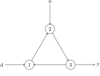
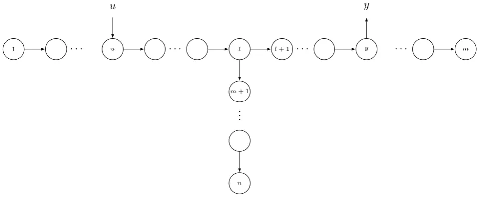
Consider the network in Figure 1, where information is shifted from vertex to vertex via the directed edges in fixed time-steps. In the vertex 3 the information can be read by the observery
and in vertex 2 an outside controller ucan change the information. Furthermore, it is possible that in every single vertex some disturbance d occurs that changes the information at that vertex. For example, in Figure 1 there is a disturbance din vertex 1.
1
2
3 y
d
[image:4.595.193.399.185.342.2]u
Figure 1: Example of a graph
We want to know if there is a control u such that the disturbance dcannot be observed by y. In other words if the disturbance dcan be counteracted by the controlleru.
Now suppose we have a similar network with one observer and one controller but withnvertices instead of 3. Again we want to know if the disturbancedacting on one vertex or multiple vertices can be counteracted by choosing the right controlu.
Formally stated our research question is:
In a network where information travels with constant speed, which is observed at a single vertex and which can be controlled at another vertex: in what subpart of the network can disturbances acting on one or multiple vertices be counteracted by the controller.
2
Problem statement and preliminaries
In systems theory the problem stated in the introduction is known as the disturbance decoupling problem (DDP) and has been solved by W. Murray Wonham and others using linear algebra, see e.g. [1, Chapter 4]. Therefore it is useful to first show the known solution to this problem for a discrete time system and then use this solution to answer the research question.
2.1 DDP for a discrete-time system
Consider the discrete time system, described by the set of equations:
x(k+ 1) =Ax(k) +Bu(k) +Sd(k) (2.1)
y(k) =Cx(k) (2.2)
wherex∈X, thestate space,u∈R and d∈R. Here x is a real vector of dimensionnand A,
B,S,C are real and constant matrices of the proper sizes.
Solving equation (2.1) for x(k) when u(k) =F x(k) and F :X →Rgives:
x(k) = (A+BF)kx(0) + k
X
i=1
(A+BF)k−iSd(i−1). (2.3)
Hence the solution for the output y(k) is:
y(k) =C(A+BF)kx(0) +C " k
X
i=1
(A+BF)k−iSd(i−1)
#
. (2.4)
Now we can define disturbance decoupling as follows.
Definition 1. The system(2.1) (2.2)is said to be disturbance decoupled if there exists a mapping
F : X → R such that for each initial state x(0) ∈ X the output y(k) is the same for every
disturbance d(·). In other words, the forced response C h
Pk
i=1(A+BF)k
−iSd(i−1)i must be
zero for the sequence d(·), and for every k= 0,1,2, . . ..
Now setting S := im (S), K := ker (C) and hA+BF |Si:= S + (A+BF)S +. . .+ (A+
BF)n−1S we arrive at the following result.
Theorem 2. By Definition 1 we have that the system (2.1), (2.2) is disturbance decoupled if and only if there exists a mapping F :X →Rsuch that:
hA+BF |Si ∈K. (2.5)
Proof. The system (2.1),(2.2) is disturbance decoupled, if and only if:
C " k
X
i=1
(A+BF)k−iSd(i−1)
#
= 0 for k= 0,1,2, . . . ∀d(·)∈R
⇔ C
" k X
i=1
(A+BF)k−iSR
#
= 0 for k= 0,1,2, . . .
⇔ C
" k X
i=1
(A+BF)k−iS
#
= 0 for k= 0,1,2, . . . .
Using the Cayley-Hamilton theorem we know that (A+BF)kfor everyk= 0,1,2, . . .is a linear combination ofI,(A+BF),(A+BF)2, . . . ,(A+BF)n−1 and soChPk
i=1(A+BF)k−iS
i
= 0 for k= 0,1,2, . . .if and only if:
C " k
X
i=1
(A+BF)k−iS
#
= 0 for k= 0,1,2, . . . , n−1
⇔ ChA+BF |Si= 0
⇔ hA+BF |Si ∈K.
2.2 Solution to the DDP in a discrete time system
The goal of this subsection is to find a solution to the disturbance decoupling problem for the system in (2.1) (2.2). In other words we want to find the ”largest” subspaceV ⊂X, such that ifS ⊂V then the system is disturbance decoupled.
By Theorem 2 we see that the subspacehA+BF |Sisatisfies two properties. FirsthA+BF |Si
is a part of the kernel ofC(hA+BF |Si ⊂K) and second if the statex(0)∈ hA+BF |Si, then (A+BF)kx(0)∈ hA+BF |Si, which means that hA+BF |Si is (A, B)-invariant.
Definition 3. A subspaceV ⊂X is(A, B)-invariant if there exists a linear mappingF :X →
R such that
(A+BF)V ⊂V. (2.6)
So we are looking for subspaces V that are (A, B)-invariant and contained in the kernel of
C. To accomplish this we construct the class J(A, B;K), containing all the (A, B)-invariant subspaces contained inK. We can define J(A, B;K) in two ways, namely via the closed loop and the open loop system.
Definition 4. J(A, B;K)cl is the class of subspaces such that V ∈ J(A, B;K)cl if and only if there is a mapping F :X →R such that for every x(0) ∈V both (A+BF)kx(0)∈V and
C(A+BF)kx(0) = 0 for k= 0,1,2, . . ..
Definition 5. J(A, B;K)ol is the class of subspaces such that V ∈J(A, B;K)ol if and only if for every x(0) ∈ V there exists a control u(k) for k = 0,1,2, . . . such that x(k) ∈ V and
y(k) =Cx(k) = 0 for k= 0,1,2, . . ..
We can show that these two definitions are equivalent by choosingu(k) =F x(k), see Theorem 28 in Appendix A.
Next we defineV∗ as the supremal element of J(A, B;K). The supremal element supB of a classBis an element inB (if it exists) such that ifV ∈B thenV ⊆supB. We can prove that the supremal element ofJ(A, B;K) exists (see Appendix A).
Theorem 6. Let V∗ be the supremal element of J(A, B;K). Then S ⊂V∗ if and only if the
Proof. SupposeS ⊂V∗. SinceV∗ is (A, B)-invariant there exists F :X →
Rsuch that (2.6)
holds. Then
hA+BF |Si ⊂ hA+BF |V∗i ⊂V∗ ⊂K.
By Theorem 2 this means that the system is disturbance decoupled.
Conversely, suppose the system is disturbance decoupled. Then there exists an F : X → R
such thathA+BF |Si ⊂K and thus hA+BF |Si ∈J(A, B;K). So:
S ⊂ hA+BF |Si ⊂V∗.
For this report V∗ = supJ(A, B;K) will be computed as in Wonham [1, Chapter 4.3], see Theorem 7.
Theorem 7. Let A : X → X, B : R → X, B = im (B) and K ⊂ X with dim(K) the
dimension of K. If we define the sequence Vµ as:
V0 =K (2.7)
Vµ=K ∩A−1 B+Vµ−1
, (2.8)
thenVµ⊂Vµ−1 and for some m≤dim(K)
Vµ= supJ(A, B;K) =V∗
(2.9)
for all µ≥m.
The operation A−1 is defined as follows by Wonham [1, Chapter 0.4]. IfV ⊂X then
A−1(V) :={x∈X |Ax∈V}. (2.10)
2.3 Constructing the feedback matrix to solve the DDP
Now that we can find V∗ the question still remains how to construct a feedback matrix
F : X → R such that (A+BF)V∗ ⊂ V∗. If F has that property we will call F a friend
of V∗ and writeF ∈F(V∗). Because u∈R we can prove F ∈F(V∗) is either unique or zero
depending onB.
Theorem 8. Let V ∈J(A, B;K). Then (a) B /∈V ⇒F is unique on V;
(b) B ∈V ⇒F = 0.
Proof. (a) Suppose F1, F2 ∈F(V). Then
That means that for every ν∈V we have
(A+BF1)ν ⊂V =ν1 ∈V, (2.11) (A+BF2)ν ⊂V =ν2 ∈V. (2.12)
Because the subspaceV is closed under addition we can subtract (2.11) en (2.12) and find (A+BF1)ν−(A+BF2)ν =ν1−ν2 ∈V
⇔BF1ν−BF2ν ∈V
⇔B(F1−F2)ν∈V.
Because B /∈V,Bu∈V if and only if u= 0 and thus
∀ν ∈V : (F1−F2)ν = 0
⇒ ∀ν ∈V : F1ν =F2ν.
Hence F is unique onV.
(b) We know thatV is (A, B)-invariant so by Lemma 29 in Appendix A AV ⊂V +B . Since
B ∈V we have
∀u∈R:Bu∈V
⇒B⊂V. (2.13)
We know AV ⊂V +B, so by 2.13 we haveAV ⊂V. This means that (A+BF)V ⊂V forF = 0.
Now following Wonham [1, Chapter 4.2] we can construct the uniqueF on V∗ as follows.
Definition 9. Let {ν1, ν2, . . . , νm}be a basis forV∗ and chooseui ∈Rsuch thatAνi =ωi−Bui
(these exist by Lemma 29 in Appendix A). We define F0 :V∗→R by
F0νi=ui for i∈ {1,2, . . . m} and ui ∈R. (2.14)
Then F0 is unique on V∗ and any linear extension F of F0 toX is a friend of V∗.
2.4 Network as a discrete time system
Now that we found a solution to the disturbance decoupling problem for a discrete time system the question remains how to solve the disturbance decoupling problem in a network such as in Figure 1. We only consider graphs with dynamics satisfying the following assumption.
Assumption 10. Graph G= (V, E) is directed and 1. G has n vertices.
3. Only one vertex vu can be controlled.
4. The controlled vertex and the observed vertex do not coincide.
5. The edge (i, j) means that (a part of ) the information that was in xi on time k is in xj
on time k+ 1.
To solve the disturbance decoupling problems in these kinds of graphs we use the structure of the graph to construct the matricesA,B and C.
We start with the construction of A. In a discrete time system the elementAji tells you how much of the information that was inxi on timekis inxj on timek+ 1, just like the edge (i, j). Therefore it makes sense to define the matrixA based on the out-degree of the vertices in the graph. Theout-degree,doutv , of vertexv is the number of edges that end inv. Now matrixA is defined as the n×n-matrix such that:
(
Aji=f(douti ) if (i, j)∈E
Aji= 0 if (i, j)∈/ E
. (2.15)
Here f is some function on the out-degree, such that f(1) = 1 and f(k) > 0 for k > 1. You can see that the value of Aij is dependent on the out-degree of vertex i. That means that if the information in isplits along multiple edges, only a part of the original information travels along each edge.
The construction of matrices B and C is fortunately a lot easier. Since we observe only at the vertex with indexy, matrixC is a row vector where they-th entry equals 1 and the othern−1 entries are zero. Similarly, matrix B is a column-vector where the u-th entry equals 1 and the other n−1 entries are zero. The 4th item of Assumption 10 implies thatB never equals CT, the transpose ofC.
For example the matrices, A,B and C in the graph of Figure 1 will be:
A=
0 0 1 1 0 0 0 1 0
,
B =
0 1 0
,
C =
0 0 1 .
To use the algorithm in Theorem 7 we also need to define the subspacesK and B.
K is the kernel of C. So K contains all the states x∈ X for which Cx = 0. Cx = 0 if and only if they-th entry of the statex is 0. Then forK we can find
K = Span{ei|i6=y}. (2.16)
In a similar manner we can findB. B is the image ofB. That meansB isB times the domain of B, which isR. Since the u-th entry is the only non-zero entry of B we find
3
Disturbance Decoupling in basic graphs
In this section Theorem 7 is used to compute V∗ for several basic graphs. These graphs all satisfy Assumption 10. Based on our observations during the computations made on these examples we will form some hypotheses that will be studied in later sections.
To make the subspaces Vµvisible in the graph, we will introduce the vertex sets Dµ andOµ.
Definition 11. Dµ is a set of vertices (Dµ⊂V) such that
{ei |i∈Dµ}
forms a basis for Vµ. In particular V∗ = Span{ei |i∈D∗}.
Please note that this definition is only valid if V∗ is indeed the span of standard unit vectors.
Definition 12. Oµ is the complement ofDµ in V.
In this section we only briefly discuss the calculation ofV∗. For a more precise computation of
V∗, we refer the reader to Appendix B.
3.1 Directed line graph
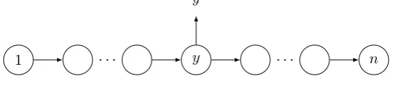
A directed line graph ~Ln is a graph G = (V, E) whose vertices can be listed in the order
{v1, v2, . . . , vn}such that: E ={(vi, vj)∈V ×V :j−i= 1}(Fagnani & Frasca [3, Chapter 2]) Now suppose we have a line-graph where vertex y is observed, see Figure 2. Note that in this figurey is both the output and the index of the observed vertex.
1 . . . y . . . n
[image:10.595.155.440.450.511.2]y
Figure 2: A directed linegraphL~n where one vertex is observed
As in Section 2.4 the structure of the graph is used to construct the matricesA,B, andC. Since there is no splitting of information we have douti = 1 and thus
(
Aji= 1 if (i, j)∈E
Aji= 0 if (i, j)∈/ E
(3.1)
A=
0 0 0 · · · 0 0 1 0 0 · · · 0 0 0 1 0 · · · 0 0
..
. . .. ... ... 0 · · · 0 1 0 0 0 · · · 0 0 1 0
C is a row-vector where they-th entry is 1 and the othern−1 entries are zero.
C =0 0 · · · 0 1
|{z}
y
0 · · · 0.
There are two spots to put the controller that might result in a fundamentally different V∗. The controller can either be on the right, uR, or on the left,uL, of the observer. Therefore we also have two differentB matrices, depending on which vertex is controlled.
Bcontrol right =
0 · · · 0 0
|{z}
y
· · · 0 1 0 · · · 0T .
Bcontrol left=
0 · · · 0 1 0 · · · 0 0
|{z}
y
· · · 0T .
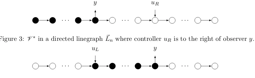
In Appendix B we used Theorem 7 to computeV∗ for both situations. The results are shown in Figures 3 and 4. There the vertices in setD∗ are white while the vertices in setO∗are black. We chose this color-coding because only disturbances occuring in the open, white, vertices and not in the closed, black, vertices can be decoupled.
. . . .
[image:11.595.162.439.182.246.2]y uR
Figure 3: V∗ in a directed linegraph ~Ln where controlleruR is to the right of observery.
. . . .
y uL
Figure 4: V∗ in a directed linegraph ~Ln where controlleruL is to the left of observery.
3.2 Directed circle graph
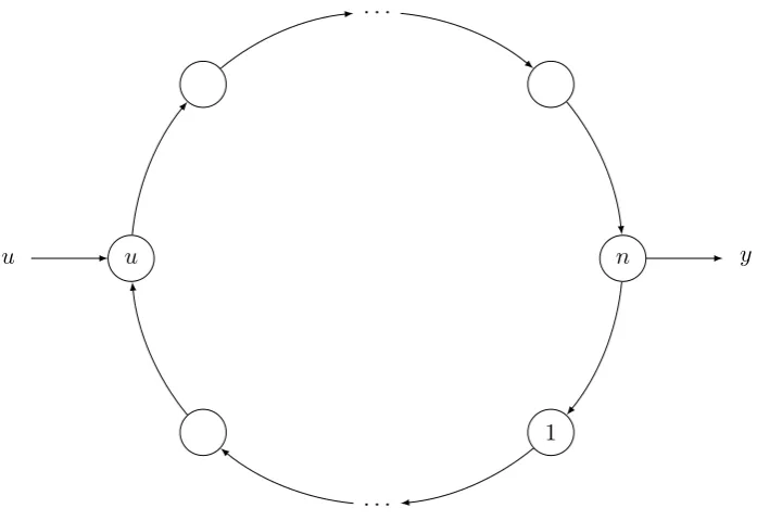
A directed circle graph C~n is a graph G = (V, E) whose vertices can be listed in the order
{v1, v2, . . . , vn} such that: E = {(vi, vj)∈V ×V :j−i= 1 mod n} (Fagnani & Frasca [3, Chapter 2]).
Now suppose that we have a directed circle graph where only the vertex n is observed and a different vertexu can be controlled, see Figure 5.
As before we used the structure of the graph to find the matrices A,B and C.
[image:11.595.88.511.319.449.2]n . . .
u
. . .
1
[image:12.595.122.471.77.317.2]y u
Figure 5: A directed circle graphC~n with one observed and one controlled vertex
A=
0 0 0 · · · 0 1 1 0 0 · · · 0 0 0 1 0 · · · 0 0 ..
. . .. ... ... 0 · · · 0 1 0 0 0 · · · 0 0 1 0
,
B =0 0 · · · 0 1
|{z}
u
0 · · · 0T,
C=0 0 0 · · · 0 1.
With these matricesA,B andC, we compute V∗ using Theorem 7 (see Appendix B). In Figure 6 you can see whatO∗ and D∗ look like. Again the white vertices are elements ofD∗ and the black vertices are elements of O∗.
3.3 Graphs where vertices have multiple outgoing edges
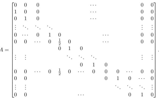
In the previous examples every vertex had only one incoming and one outgoing edge. It might be interesting to see what happens if one or more vertices have multiple outgoing edges. As an example we chose the graph G~split of Figure 7. In that graph there is a vertex l with two outgoing edges, (l, l+ 1) and (l, m+ 1).
. . .
. . .
[image:13.595.209.384.75.206.2]y u
Figure 6: V∗ in a directed circle graph C~n with one observed and one controlled vertex
1 · · · u · · · l l+ 1 · · · y · · · m
m+ 1
.. .
n
u y
Figure 7: GraphG~split where vertexlhas two outgoing edges, vertexu is controlled and vertex
y is observed.
Thus we define A as follows:
Aji = 12 ifi=l and (l, j)∈E
Aji = 1 ifi6=l and (i, j)∈E
Aji = 0 elsewhere
[image:13.595.69.551.248.450.2]Using equation (3.2) the matrixA is as follows. A=
0 0 0 · · · 0 0
1 0 0 · · · 0 0
0 1 0 · · · 0 0
..
. . .. ... ... ... ...
0 · · · 0 1 0 · · · 0 0
0 0 · · · 0 12 0 · · · 0 0
0 1 0
..
. ... . .. ... ... ... ...
0 1 0
0 0 · · · 0 12 0 · · · 0 0 0 · · · 0 0
0 0 0 1 0 · · · 0
..
. ... . .. ... ... ...
0 0 · · · 0 1 0
.
Matrix B is a column-vector where only theu-th entry, between the first and thel-th entry, is non-zero and equal to 1.
B =
0 · · · 0 1
|{z}
u
0 · · · 0 0
|{z}
l
0 · · · 0T .
MatrixC is just as in Section 3.1 a row-vector where they-th entry, between thel-th and m-th entry, is 1 and the other n−1 entries are zero.
C=
0 0 · · · 0 0
|{z}
l
0 · · · 0 1
|{z}
y
0 · · · 0 0
|{z}
m
0 · · · 0 .
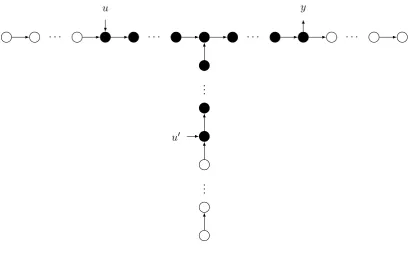
For these matrices V∗ is computed in Appendix B. The results can be seen in Figure 8 where the elements of D∗ are white and the elements of O∗ black.
· · · ·
.. .
[image:14.595.140.456.94.292.2]y u
Figure 8: V∗ in graph G~split.
3.4 Graphs where vertices have multiple incoming edges
1 · · · u · · · l−1 l l+ 1 · · · y · · · m
n
.. .
m+ 1
[image:15.595.61.551.73.279.2]u y
Figure 9: Graph G~incoming where vertex l has two incoming edges, vertex u is controlled and vertex y is observed.
In this graph there is no splitting of information and we can use the definition for matrix Ain (3.1) to construct the following matrix. This matrix is slightly different from the matrix A in Section 3.1 because rowl+ 1 has a second non-zero entry ((A)l+1,n = 1) and rowm+ 1 consists entirely of zeros.
A=
0 · · · 0 0
1 0 · · · 0 0
0 1 0 · · · 0 0
..
. . .. ... ... ... ...
0 · · · 0 1 0 · · · 0 0
0 · · · 0 1 0 · · · 0 1
0 · · · 0 1 0 · · · 0 0
..
. . .. ... ... ... ...
0 · · · 0 1 0 · · · 0 0
0 · · · 0 0 0 · · · 0 0
0 · · · 0 1 0 · · · 0 0
..
. . .. ... ... ... ...
0 · · · 0 1 0 0
0 · · · 0 1 0
MatrixBis still a column-vector where only theu-th entry, between the first and thel-th entry, is non-zero and equal to 1.
B=
0 · · · 0 1
|{z}
u
0 · · · 0 0
|{z}
l
0 · · · 0T
other n−1 entries are zero.
C=0 0 · · · 0 0
|{z}
m
0 · · · 0 1
|{z}
y
0 · · · 0.
The computation forV∗ with these matrices can be found in Appendix B again.
However in this case V∗ is not the span of unit vectors, so we do not have the vertex sets D∗
and O∗. Instead, we introduce two new vertex setsDµand Oµ.
Definition 13. Let Eµ be the largest span of unit vectors, such that Eµ⊂Vµ. Then i∈Dµ if
and only if ei∈Eµ. In particular E∗ is the largest span of unit vectors such that E∗⊂V∗.
Definition 14. Oµ is the complement of Dµ in V.
In Figure 10 we visualizedD∗andO∗by coloring the vertices inD∗white and the vertices inO∗
black. Here u0 is a vertex such that d(u0, l) =d(u, l). Hered(i, j) is defined asthe distance, the length of shortest path between vertex iandj. That means that the path fromu0 tol has the same length as the path fromutol. If however there is no suchu0, becaused(m+ 1, l)< d(u, l) the entire path (m+ 1, n) belongs to O∗ and is subsequently colored black.
· · · ·
.. .
.. .
y u
[image:16.595.91.503.332.585.2]u0
Figure 10: V∗ in graph G~incoming.
3.5 Observations made during the computation
While computing V∗ for these examples we made several observations in the graph, see also Appendix B. We give a summary of these observations.
However, if there is a vertex with more than one incoming edge, V∗ is not the span of unit vectors. In that case, we saw that all the vertices that cannot reach vertex y are contained in
Dµ. Also if there exists a vertex u0 such that d(u0, y) is equal tod(u, y) then only the shortest paths fromu toy and u0 toy are contained in O∗.
4
Relationship between disturbance decoupling and the graph
structure
In this section we will prove or disprove several theorems regarding V∗ of graphs that satify Assumption 10.
4.1 Unobservable subspace
The unobservable subspace of a system is the subspace N containing all inital states x where the uncontrolled outputy is zero at every time k= 0,1,2,3, . . .. (Meinsma [2])
N =
n
x(0)∈X |CAkx(0) = 0 ∀k= 0,1,2,3, . . . o
(4.1)
It is immediately clear thatN ⊂K . Now we prove thatN is also an (A, B)-invariant subspace.
Lemma 15. The unobservable subspace N is(A, B)-invariant.
Proof. Let x(0) be an arbitrary element ofN . By definition ofN we have
CAkx(0) = 0∀k= 0,1,2, . . . . (4.2)
Now chooseF = 0, then (A+BF)x(0) =Ax(0) and we have
∀k= 0,1,2, . . .: CAkAx(0) =CAk+1x(0) = 0 according to (4.2). This means thatAx(0)∈N.
Since x(0) was arbitrary we have found anF :X →R (F = 0) such that for everyx(0)∈N,
(A+BF)x(0)∈N . SoN is (A, B)-invariant.
Now it is easy to prove that the unobservable subspace is contained in V∗.
Theorem 16.
N ⊂V∗.
Proof. N is a subspace that is contained inK and by Lemma 15N is (A, B)-invariant. Since
V∗ is the supremal element of the class with these two properties we have N ⊂V∗.
Definition 17. Let G=(V,E) be a graph satisfying Assumption 10 and lety be the index of the observed vertex. VN ⊂ V is the subset of vertices such that v ∈ VN if and only if there is no
path from v toy.
Theorem 18. Let G = (V, E) be a graph satisfying Assumption 10 where the observer has index y and V∗ = Span{ei |i∈D∗}, then
VN ⊂D∗.
Proof. By Lemma 32 in Appendix A we know (Ayi)k = 0 for every i∈ VN for k = 0,1,2, . . .. Then for i∈VN
∀k= 0,1,2, . . . CAkei =C
(Ak) 1i (Ak)2i
.. . (Ak)yi
.. . (Ak)ni
= (Ak)yi= 0
and thus ei ∈N for every i∈VN.
Because a subspace is closed under addition and scalar multiplication that means Span{ei |i∈VN} ⊂N.
Theorem 16 implies
Span{ei |i∈VN} ⊂N ⊂V∗ = Span{ei |i∈D∗}
⇒Span{ei|i∈VN} ⊂Span{ei|i∈D∗}
⇒VN ⊂D∗.
4.2 Out-neighbours
In the graph G= (V, E), satisfying Assumption 10, v is anout-neighbour ofw if (w, v)∈E, in which casev ∈Nout(w). In that case w is anin-neighbour of v and w∈Nin(v)
Nout(w) ={v∈V |(w, v)∈E}, (4.3)
Nin(v) ={w∈V |(w, v)∈E}. (4.4)
As seen in the previous examples there seems to be a relation between the out-neighbours of vertices and theV∗-algorithm. To prove this we will use the properties of the A-matrix.
Lemma 19. Let G = (V, E) be a graph satisfying Assumption 10 with matrix A as in (2.15)
and let ew be a standard unit vector. Then for all w in V, Aew is a column-vector where the
Proof. By matrix multiplication, we know:
Aew =
A1w
A2w .. .
Avw .. .
Anw
. (4.5)
By definition of matrixAin (2.15) we knowAvw = 0 if and only if (w, v) is not inE. SoAew is a column-vector where the v-th entry is zero if and only if vis not an out-neighbour of w. The converse of this statement completes the proof.
Using this property of Aew we can use out-neighbours to determine the next step in the V∗ -algorithm.
Theorem 20. Let G= (V, E) be a graph satisfying Assumption 10 and let vertex w be in V, such that w is not the observed vertex. Now if Vµ is the subspace after µ iterations of the
V∗-algorithm, Vµ= Span{e
i |i∈Dµ} andB ⊂Vµ, then
Nout(w)⊂Dµ⇔w∈Dµ+1.
Proof. SupposeNout(w)⊂Dµ then by the definition ofDµ
Span
ei|i∈Nout(w) ⊂Span{ei |i∈Dµ}=Vµ.
By Lemma 19 Aew is a column vector where the i-th entry is non-zero if and only if i is an out-neighbour ofw. That means
Aew ∈Span
ei |i∈Nout(w)
⇒Aew ∈Vµ. (4.6)
Since wis not the observed vertex we have ew∈K ⊂X and by (A.3) we get
ew∈A−1(Vµ+B)
⇒ew ∈K ∩A−1(Vµ+B)
⇒ew ∈Vµ+1= Span
ei|i∈Dµ+1 .
Finally, by the definition ofDµ+1 we have
w∈Dµ+1.
Conversely, suppose w∈Dµ+1. Then by definition of Dµ+1 and Theorem 7
ew ∈Vµ+1
⇒ew ∈K ∩A−1(Vµ+1+B)
⇒ew ∈A−1(Vµ)
NowAew is a column-vector where thei-th entry is non-zero if and only ifiis an out-neighbour of w. That means that
Aew =
X
i∈Nout(w)
aiei∈Vµwith ai ∈R\ {0}
⇒ei ∈Vµ ∀i∈Nout(w)
⇒Span
ei |i∈Nout(w) ⊂Vµ= Span{ej |j ∈Dµ}
⇒Nout(w)⊂Dµ.
This is an interesting result but it doesn’t tell us how a controlled vertex will influence the V∗. The next result will tell us something about that.
Theorem 21. Suppose Vµ is the subspace afterµ iterations of theV∗-algorithm. Then, if
Vµ+B=Vµ−1
⇒Vµ=V∗. (4.7)
Proof. We know
Vµ+1=K ∩A−1(Vµ+B) =K ∩A−1(Vµ−1).
NowVµ+B=Vµ−1 also means B⊂Vµ−1 and:
Vµ+1=K ∩A−1(Vµ−1+B) =Vµ.
So Vµ=V∗ proving the result.
In a graph we can visualize this as follows
Theorem 22. Suppose Vµ is the subspace after µiterations of the V∗-algorithm and u is the index of the controlled vertex. IfDµ+u=Dµ−1 then Dµ=D∗.
Proof. If Dµ+u=Dµ−1 we know
Vµ+B= Span{e
i |i∈Dµ}+ Span{eu} = Span{ei |i∈Dµ+u}
= Spanei |i∈Dµ−1 =Vµ.
So by Theorem 21, Vµ=V∗ and Dµ=D∗.
5
Solving the DDP based on the graph structure
5.1 Graphs where the vertices have a maximum in-degree of 1
In this paragraph we will restrict ourselves to graphs where each vertex has an in-degree of 1 or less (din
v ≤1). As we have seen in section 4 some theories rely on the fact thatB⊂N . There-fore it might be interesting to see how we can solve the DDP in graphs where the controlled vertex ulies in VN. Since in that case B= Span{eu} ⊂Span{ei|i∈VN}.
Theorem 23. Suppose G= (V, E) is a graph with the given properties, u is the index of the controlled vertex andu∈VN. Then
D∗ =VN.
Proof. According to Theorem 18VN ⊂D∗. So we only need to proveD∗ ⊂VN or that ifv∈D∗ thenv∈VN. We will prove the converse statement.
v /∈VN ⇒v /∈D∗.
Lety be the index of the observed vertex and suppose v /∈VN. Then by definition ofVN there is a pathP fromv toy. We will provev /∈D∗ via induction on the lengthm of P.
We start with m= 0. In that casev=y and it is clear thatv /∈D∗.
Nowo suppose that if there is pathP of lengthm from vertexv toy, thenv /∈D∗.
Letv be a vertex such that (v, v2, v3, . . . , vm, y) is the shortest path fromv toy. The length of this path is m+ 1. Clearly there is a path (v2, v3, . . . , vm, y) of length m from v2 to y and by the induction hypothesis we havev2 ∈/D∗. In that casev has a neighbourv2 that is not inD∗ soNout(v)6⊆D∗. Then by Theorem 20v /∈D∗.
So via induction we have proven that if there is path from v to y (v /∈ VN) then v /∈ D∗. So
D∗ ⊂VN and D∗=VN.
Because u is an element of VN =D∗,B =eu ∈V. Therefore according to Theorem 8, we can choseF, the feedback matrix to solve the DDP, to be zero.
Now that we have shown what happens ifu∈VN, see Theoren 23, we assume in the remaining of this paragraph thatu /∈VN.
Lemma 24. Let G= (V, E) be a graph satisfying Assumption 10 with dinv ≤1 for every v∈V
and u /∈VN. Then there is a unique path fromu toy.
Theorem 25. Let G = (V, E) be a graph satisfying Assumption 10 with dinv ≤ 1 for every
v ∈ V, u /∈ VN and P the unique path from the controlled vertex u to the observed vertex y,
then
P =O∗ (5.1)
Proof. First we renumber the vertices such that P = {u, u−1, . . . ,2,1,0 = y}. So for i ∈ {0,1,2, . . . , u−1, u}we have (Ax)i =ai+1xi+1andai+1 >0. Please note that only in this proof the first row ofA has index 0.
Via induction we prove that Oµ={0,1, . . . , µ} for 0≤µ≤u. Forµ= 0 we have
V0 =K = Span{ei |i6=y} (5.2)
⇒D0 =V \ {y} ⇒O0 ={y}={0}.
and the statement holds forµ= 0. Now suppose the statement holds for some µ=µ0≤u−1.
Oµ0 ={0,1, . . . , µ
0}
⇒Dµ0 =V{0,1, . . . , µ
0}
⇒Vµ0 = Span{e
i|i /∈ {0,1, . . . , µ0}}. (5.3) Nowµ0 ≤u−1 implies i≤µ0 < uwhich means B⊂Vµ0 and so B+Vµ0 =Vµ0. Thus
Vµ0+1=K ∩A−1(Vµ0). (5.4)
By (2.16) we knowK and by (2.10) we knowA−1(Vµ0) ={x∈X |Ax∈Vµ0}. Now by (5.3) Ax∈Vµ0 ⇔(Ax)
i= 0 for i∈ {0,1, . . . , µ0}
⇔ai+1xi+1= 0 for i∈ {0,1, . . . , µ0}
⇔xi+1= 0 for i∈ {0,1, . . . , µ0}, where we have used ai+1 >0 and so
x∈A−1(Vµ0)⇔x
µ0+1=· · ·=x2 =x1 = 0
⇒x∈K ∩A−1(Vµ0)⇔x
µ0+1=· · ·=x2=x1 =x0 = 0
Now by (5.4) we have
Vµ0+1=K ∩A−1(Vµ0) = Span{e
i |i /∈ {0,1,2, . . . , µ0+ 1}}
⇒Dµ0+1=V \ {0,1,2, . . . , µ
0+ 1}
⇒Oµ0+1={0,1,2, . . . , µ
0+ 1}.
So via induction we have proven that the statement is true for 0 ≤ µ ≤ u. In particular
Ou = {0,1,2, . . . , u}= P. So now we have to prove Ou =O∗. Using Theorem 22 and Oµ we have
Du+u= (V \ {0,1,2, . . . , u}) +u=V \ {0,1,2, . . . , u−1}=Du−1
⇒Du =D∗
⇒Ou =O∗.
In this graph we also have a unique feedback matrixF onV∗.
Theorem 26. Let G = (V, E) be a graph satisfying Assumption 10 with dinv ≤ 1 for every
v ∈ V, u /∈ VN and P the unique path from the controlled vertex u to the observed vertex y.
Then if u has an incoming edge (u+ 1, u), F = (−eu+1)T is a feedback matrix unique on V∗
such that V∗ is (A, B)-invariant.
Proof. Let {ei |i ∈D∗} be a basis for V∗. Now if Aei+BF ei ∈V∗ for all i∈D∗ then F is the feedback matrix unique onV∗ such that V∗ is (A, B)-invariant.
Take O∗ = P = {u, u−1, . . . ,2,1,0 = y}. Because for every i ∈ V we have dini ≤ 1 also
|Nin(i)| ≤1. Then for everyi∈P,i6=u we have
Nin(i) ={i+ 1} ∈O∗.
That means u is the only vertex in O∗ with an out-neighbor in D∗ (namely u+ 1) and thus
u+ 1 is the only vertex inD∗ with an in-neighbor inO∗.
Now by Lemma 19, Aei is a column vector where the v-th entry is non-zero if and only if v is an out-neighbour of i. So for everyi∈D∗\ {u+ 1} we have
Aei ∈Span
ev|v∈Nout(i) ⊂Span{ej |j∈D∗}
⇒Aei∈V∗.
ChoosingF = (−eu+1)T we haveF ei = 0 fori∈D∗\ {u+ 1}which implies that Aei+BF ei=
Aei+B·0 =Aei ∈V∗.
For i = u+ 1 we know that u + 1 has one neighbour u in O∗ and an unknown number of neighbours in D∗. So for ai ∈R we have
Aeu+1=eu+
X
i∈D∗
aiei.
Now choosing F = (−eu+1)T we have F ·eu+1 = −1 and by Assumption 10 we have B = eu, which we get
Aeu+1+BF eu+1 =
X
i∈D∗
aiei+eu+eu· −1
= X i∈D∗
aiei ∈Span{ei |i∈D∗}=V∗
which means thatAeu+1+BF eu+1∈V∗ and we have proven thatF = (−eu+1)T is a feedback matrix unique onV∗ such that V∗ is (A, B)-invariant.
5.2 General graphs
In this paragraph we look at an arbitrary graph satisfying Assumption 10. In this case it is possible, that V∗ is not the span of standard unit vectors. Therefore we cannot use Theorem 18 and Theorem 20 in Section 4. However, in Appendix A we have proven a similar theorems using D∗.
Theorem 27. Let graph G= (V, E) satisfy Assumption 10. Then for v∈V we have (a) v∈VN ⇒ev ∈V∗.
(b) d(v, y)< d(u, y)⇒ev ∈/V∗.
(c) d(v, y) =d(u, y)⇒ev ∈/V∗.
(d) If for every v∈V satisfyingd(v, y) =d(u, y) + 1there holdsev ∈V∗ thend(v, y)> d(u, y)
implies that ev ∈V∗.
Proof. (a) By the proof of Theorem 33 we have for v∈VN. ev ∈N ⊂V∗. (b) First we prove via induction for 0≤µ < d(u, y) that
Oµ={v∈V |0≤d(v, y)≤µ}. (5.5)
B⊂Vµ. (5.6)
Forµ= 0 we have
V0 =K = Span{e
i|i6=y}.
In this caseV0 is the greatest span of unit vectors inV0 and thus
⇒D0=V \ {y}
⇒O0={y}.
Since {v ∈ V | d(v, y) = 0} = {y}, (5.5) holds for µ = 0. Furthermore, B = Span{eu} ⊂ Span{ei|i6=y}=V0 so (5.6) holds as well forµ= 0.
Now assuming (5.5) and (5.6) hold forµ, we can prove that (5.5) and (5.6) also hold forµ+ 1. Letvbe an arbitrary vertex withd(v, y) =µ+ 1. That means there is a pathP = (v, v1, . . . , y) of length µ+ 1. Then there is path (v1, . . . , y) of length µ from v1 to y which means that
d(v1, y)≤µso by the induction hypothesis v1∈Oµ and subsequently v1∈/ Dµ.
Now v has the out-neighbour v1 ∈/ Dµ so Nout(v) 6⊂ Dµ. Since B ⊂Vµ we can use Theorem 34 and thenNout(v)6⊂D
µimplies v /∈Dµ+1 sov ∈Oµ+1. v was an arbitrary vertex and hence (5.6) holds forµ+ 1.
Moreover, {ei | d(i, v) > µ+ 1} ⊂ {ei | i /∈ Oµ} = {ei | i ∈ Dµ} ⊂ Vµ+1. By assumption
d(u, v)> d(v, y) =µ+ 1 soeu∈Vµ+1. HenceB= Span{eu} ⊂Vµ+1 and thus (5.6) also holds forµ+ 1.
We have now proven that if d(v, y) < d(u, y), then v ∈ Od(v,y) and since Oµ ≤Oµ+1 we have
Span{ei |i∈D∗}is the greatest span of unit vectors contained in V∗ this means thatev ∈/ V∗ completing the proof.
(c) In part (b) we saw that Oµ={v∈V |0≤d(v, y)≤µ} and B⊂Vµ forµ < d(u, v). Letd(u, v) =m, thenm−1< d(u, v) and
Om−1 ={v∈V |0≤d(v, y)≤m−1} (5.7)
B⊂Vm−1. (5.8)
Now letvbe an arbitrary vertex withd(v, y) =mand let P = (v, v1, . . . , y) be a path of length
m from v to y. Then there is a path (v1, . . . , y) of length m−1 from v1 to y. This means that d(v1, y) ≤ m−1 < m = d(u, y) and by (5.7) v1 ∈ Om−1 and thus v1 ∈/ Dm−1. Since
v1 ∈Nout(v), we haveNout(v)6⊂Dm−1. By (5.8) we can use Theorem 34 so
v /∈Dm
⇒v /∈D∗.
Again because Span{ei |i∈D∗}is the greatest span of unit vectors contained inV∗this means
thatev ∈/V∗.
(d) We prove that for everyv∈V satisfying d(v, y)> d(u, y),ev ∈Vµ forµ= 0,1,2, . . .. Forµ= 0 we havev 6=y and thus ev ∈K =V0.
Now suppose that ev ∈ Vµ0 for every v ∈ V satisfying d(v, y) > d(u, y). We prove that
ev ∈Vµ0+1.
By assumption we have that if d(v, y) =d(u, y) + 1 thenv∈V∗ and thus v∈Vµ0+1.
So all that is left to prove is that ev ∈Vm0+1 for every v ∈V satisfying d(v, y)> d(u, y) + 1. We know that
Vµ0+1=K ∩A−1(Vµ0+B).
When d(v, y) > d(u, y) + 1, we have v 6=y and thus ev ∈ K. So we only need to prove that
ev ∈A−1(Vµ0 +B).
A−1(Vµ0+B) ={x∈X |Ax∈Vµ0+B}. By Lemma 19Ae
i is a vector where thej-th entry is non-zero if and only ifjis an out-neighbour ofi. Now forvwithd(v, y)> d(u, y) + 1, we have for every out-neighbourw ofvthatd(w, y)> d(u, y) and by induction hypothesisew ∈Vµ0 for everyw∈V satisfying d(w, y)> d(u, y). Then
Aev ∈Span
ew |w∈Nout(v) ⊂Span{ej |d(j, y)> d(u, y)} ⊂Vµ0.
So we have Aev ∈ Vµ0 +B and thus ev ∈A−1(Vµ0 +B). Combining this with ev ∈K, we have proven thatev ∈Vµ0+1.
So for every v ∈ V satisfying d(v, y) > d(u, y) we have that ev ∈ Vµ for µ = 0,1, . . ., which meansev ∈V∗.
span of standard unit vectors (E∗ = Span{ei |i∈D∗}) contained inV∗. That means that every
disturbance acting on one or multiple vertices in D∗ can be decoupled. It is also important to
note that sinceE∗ ⊂V∗, it is possible that a disturbance acting on some other vertices that are not elements of D∗ can also be decoupled.
6
Conclusion
Our research question was: In a network where information travels with constant speed, which is observed at a single vertex and which can be controlled at another vertex: in what subpart of the network can disturbances acting on one or multiple vertices be counteracted by the controller?
This problem is known as the disturbance decoupling problem (DDP) in systems theory. Hence we combined theorems in literature [1, Chapter 4] regarding the disturbance decoupling problem with graph theory by providing a method to rewrite graphs as discrete time systems. This way we were able to solve the problem for a few basic graphs. However these computations were complex and lenghty and the results were only relevant for a very small group of graphs. However we could solve the problem for a larger group of graphs, by using the observations we made during these computations.
To achieve this result, we created two groups of graphs, thereby creating two sub problems from the research question. (1) how to solve the disturbance decoupling problem in a network where vertices cannot have multiple incoming edges are not allowed and (2) how to solve the distur-bance decoupling problem in networks where vertices are allowed to have multiple incoming edges.
We have found a solution to the first subproblem, for graphs where vertices cannot have multiple incoming edges. For these graphs we showed how to construct a subset of verticesD∗ such that a disturbance can be decoupled if and only if that disturbance acts on one or multiple vertices of this subset.
For the second problem we only managed to find a partial solution. For these graphs, we can create another subset D∗ such that if a disturbance acts on one or multiple vertices of this
subset then it can be decoupled. This means that it is possible that there are more types of disturbances that can also be decoupled, which we did not find. Moreover, we can only create
D∗if an extra assumption is fulfilled. We do have a strong suspicion that this assumption holds
for every graph but that remains to be proven. So in order to find every type of disturbance that can be decoupled in an arbitrary graph further research is required.
We can also continue the research in other areas. On the one hand we could develop an algorithm to solve the problem for very large graphs using a computer. On the other hand we could use the knowledge we gained by solving the disturbance decoupling problem where the control is fixed on one vertex to figure out how to place the controller in the network such that the maximum amount of disturbances can be decoupled.
7
Overview of all symbols and notations
To help the reader we have compiled a list of the notations and symbols that are used.
• A:X →X • B :R→X
• C:X →R • S:R→X
• F :X →R
• AT := the transpose of matrixA
• S := im (S)
• B:= im (B)
• K := ker (C)
• dimV := the dimension of subspaceV
• V := set of all the nodes in graphG= (V, E)
• E := set of all the edges in graphG= (V, E)
• |V|:= the cardinality of set V
• n:= |G(V)|
• x(k) := statex on timek
• xi := the i-th element of state x
• N ⊂X := the unobservable subspace
• VN := the subset of vertices that have no path to the observer y
• d(v, w) := the length of the path between v andw
• J(A, B;K) := the class of (A, B)-invariant subspaces contained in K
• hA+BF|Si:=S + (A+BF)S +. . .+ (A+BF)n−1S
• A−1(V) :={x∈X|Ax∈V} • ei := the standard unit vector
• douti := the out-degree of vertexi
• dini := the in-degree of vertexi
• Nout(i) := the subset of out-neighbors of vertexi
• Nin(i) := the subset of in-neighbors of vertexi
• Dµ := the set of vertices such that{ei|i∈Dµ} forms a basis forVµ
• Oµ := the complement of Dµin V
• Dµ := the set of vertices such thatSpan{ei|i∈Dµ}is the largest span of unit vectors in
Vµ
References
[1] Wonham, W.M. (1985). Linear Multivariable Control: A Geometric Approach (3rd ed.). New York, NY: Springer-Verlag.
[2] Meinsma, G. (2015). Inleiding wiskundige systeemtheorie. Enschede: Universiteit Twente. [3] Fagnani, F. & Frasca, P. (2014). Introduction to Averaging Dynamics over Networks (1st
Appendices
A
Proofs
Theorem 28. Let V be a subspace. Then
V ∈J(A, B;K)cl ⇔V ∈J(A, B;K)ol
Proof. Suppose V ∈J(A, B;K)cl that means there exists a linear mapping F :X → Rsuch
that that for everyx(0)∈V andk= 0,1,2, . . .
(A+BF)kx(0)∈V
C(A+BF)kx(0) = 0
Letx(0) be an arbitrary element ofV. For k= 0 we know
x(0)∈V
y(0) =Cx(0) =C(A+BF)0x(0) = 0.
That means thatx(0)∈V and y(0) = 0. Fork= 1 choose u(0) =F x(0).
x(1) =Ax(0) +Bu(0) =Ax(0) +BF x(0) = (A+BF)x(0)∈V
y(1) =Cx(1)
=C(A+BF)x(1) = 0
That means that there exists au(0) such thatx(1)∈V andy(1) = 0.
Now suppose for k that there is a u such that x(k)∈V and y(k) = 0. Then for k+ 1 choose
u(k) =F x(k).
x(k+ 1) =Ax(k) +Bu(k) =Ax(k) +BF x(k) = (A+BF)x(k)∈V
y(k+ 1) =Cx(k+ 1)
=C(A+BF)x(k) = 0
Since x(0) was chosen at random we know that for every x(0) there is a u(k) fork= 0,1,2, ...
such thatx(k)∈V andy(k) = 0. So V ∈J(A, B;K)ol.
Conversely, suppose V ∈ J(A, B;K)ol. That means that for every x(0) ∈ V there is a u(k) such thatx(k)∈V andy(k) = 0. Now let{ν1, ν2, . . . , νµ} be a basis forV. Then for every νi, fori= 0,1,2, . . . , µthere is a controlui such that
Aνi+Bui∈V (A.1)
DefineF0 :X →RbyF0νi =ui and letF be some linear extension of F0 toX. We prove via induction that (A+BF)kν
i ∈V and C(A+BF)kνi= 0. For k= 0 we have (A+BF)0νi=νi∈V
C(A+BF)0νi=Cνi = 0
And suppose for k=swe have (A+BF)sνi ∈V and C(A+BF)sνi= 0.
Since (A+BF)sνi ∈V we have (A+BF)sνi=Pi∈{0,1,...,µ}aiνiwithai ∈R. Then fork=s+1:
(A+BF)s+1νi= (A+BF)(A+BF)sνi = (A+BF) X
i∈{0,1,...,µ}
aiνi
= X
i∈{0,1,...,µ}
ai(A+BF)νi
= X
i∈{0,1,...,µ}
ai(Aνi+BF νi)
= X
i∈{0,1,...,µ}
ai(Aνi+Bui)
We know by (A.1) that Aνi+Bui ∈V. Since subspace V is closed under addition and scalar multiplication this means P
i∈{0,1,...,µ}ai(Aνi+Bui) ∈ V and so (A+BF)s+1νi ∈ V. Then also (A+BF)s+1νi=Pi∈{0,1,...,µ}biνi withbi ∈R. Combining this with (A.2) we have
C(A+BF)s+1νi=C
X
i∈{0,1,...,µ}
biνi
= X
i∈{0,1,...,µ}
biCνi
= X
i∈{0,1,...,µ}
bi·0 = 0
So we have proven for k= 0,1,2, . . . that for everyνi withi∈ {0,1, . . . , µ} (A+BF)kνi ∈V
C(A+BF)kνi= 0
And since this holds for a basis of V we have constructed a linear mapping F :X → Rsuch
that for every x(0)∈V fork= 0,1,2, . . .
(A+BF)kx(0)∈V
C(A+BF)kx(0) = 0 which means thatV ∈J(A, B;K)cl.
Lemma 29. Let V ⊂K and B= im (B). Then
V ∈J⇔AV ⊂V +B
Proof. SupposeV ∈Jand letν ∈V. By definitionV is (A, B)-invariant and so (A+BF)ν =ω
for someω∈V. Thus
Aν =ω−BF ν ⇒Aν ∈V +B.
Since ν is arbitrary this means that Aν ∈V +B for everyν ∈V and thus AV ⊂V +B. Conversely, letV ⊂K be a subspace such thatAV ⊂V +B and let{ν1, ν2, . . . , νµ}be a basis forV. Then for every νi, fori= 0,1,2, . . . , µ there exist aωi ∈V andui∈Rsuch that
Aνi=ωi−Bui
Now define F0 :X →Rby F0νi=ui and let F be some linear extension of F0 toX. Then
Aνi =ωi−BF νi
Aνi+BF νi =ωi (A+BF)νi =ωi
And since this holds for a basis ofV we know (A+BF)V ⊂V ⊂K. So V ∈J.
Lemma 30. J is closed under the operation of subspace addition.
Proof. Let V1,V2 ∈J. Then by Lemma 29
AV1⊂V1+B, and
AV2⊂V2+B.
Thus A(V1+V2) =A(V1) +A(V2) ⊂V1+V2+B. Now by Lemma 29 we know V1+V2 ∈ J and so Jis closed under the operation of subspace addition.
Theorem 31. supJ exists.
Proof. First we will prove that the supremal element of J exists. We know that J is a class of subspaces of K and since K is finite-dimensional there must be an element V∗ of greatest dimension. Now let V be an arbitrary element ofJ. We haveV +V∗∈J, because by Lemma 30 J is closed under the operation of subspace addition. Now let dim(V) be the dimension of subspaceV, then
dim(V∗)≥dim(V +V∗)≥dim(V∗).
That means thatd(V∗) =d(V +V∗) and thusV∗=V∗+V, which means thatV ⊂V∗. Since V was arbitrary this holds for every subspace V ∈J and so V∗ = supJexists.
Now we will show that V∗ is unique. Suppose there is another supremal element V. By definition of the supremal elementV ∈J soV ⊂V∗. Also V∗ ∈J so V∗ ⊂V. Which means
Lemma 32. Let G = (V,E) be a graph satisfying Assumption 10 and matrix A defined as in
(2.15). Then for all v, w∈V andk= 1,2, . . . if there is no path from v to w then(Ak)
wv= 0.
Proof. The statement is proven by induction on k. By the definition of matrix Ain (2.15) this is true fork= 1.
Now we suppose the statement is true forkand we will prove it is also true fork+ 1. We know that if the edge (v, i) exists there is no path from itow (otherwise there would be a path from
v tow).
(Ak+1)wv=X i∈V
(Ak)wiAiv
= X
i∈V|(v,i)∈E
(Ak)wiAiv+
X
i∈V|(v,i)∈/E
(Ak)wiAiv
= X
i∈V|(v,i)∈E
0·Aiv+
X
i∈V|(v,i)∈/E
(Ak)wi·0
= 0 + 0 = 0.
So by induction the statement is true for allk= 1,2, . . .
Theorem 33. Let G = (V, E) be a graph satisfying Assumption 10 where the observer has index y, then
VN ⊂D∗.
Proof. By Lemma 32 in Appendix A we know (Ayi)k = 0 for every i∈ VN for k = 0,1,2, . . .. Then for i∈VN
∀k= 0,1,2, . . . CAkei =C
(Ak)1i (Ak)
2i .. . (Ak)yi
.. . (Ak)ni
= (Ak)yi= 0
and thus ei ∈N for every i∈VN.
Because a subspace is closed under addition and scalar multiplication that means by Theorem 16
Span{ei |i∈VN} ⊂N ⊂V∗
Now sinceE∗ is the largest span of unit vectors such that E∗ ⊂V∗ we have Span{ei |i∈VN} ⊂E∗ = Span{ei |i∈D∗}
⇒Span{ei |i∈VN} ⊂Span{ei |i∈D∗}
⇒VN ⊂D∗
Theorem 34. Let G = (V, E) be a graph satisfying Assumption 10 and let vertex w ∈ V, not the observed vertex. Now if Vµ is the subspace after µ iterations of the V∗-algorithm and B⊂Vµ, then
Nout(w)⊂Dµ⇔w∈Dµ+1
Proof. SupposeNout(w)⊂Dµ then by the definition of Dµ
Spanei |i∈Nout(w) ⊂Span{ei |i∈Dµ} ⊂Vµ.
By Lemma 19 Aew is a column vector where the i-th entry is non-zero if and only if i is an out-neighbour ofw. That means
Aew ∈Span
ei |i∈Nout(w)
⇒Aew ∈Vµ (A.3)
Since wis not the observed vertex we have ew∈K ⊂X and by (A.3) we get
ew ∈A−1(Vµ+B)
⇒ew ∈K ∩A−1(Vµ+B)
⇒ew ∈Vµ+1
And sinceEµ+1 is the largest largest span of unit vectors in Vµ we have
ew ∈Eµ+1 = Span{ei|i∈Dµ+1}
⇒w∈Dµ+1
Conversely, suppose w∈Dµ+1. Then by definition of Dµ+1 and Theorem 7
ew ∈Eµ+1⊂Vµ+1
⇒ew ∈Vµ+1
⇒ew ∈K ∩A−1(Vµ+1+B)
⇒ew ∈A−1(Vµ)
⇒Aew∈Vµ
NowAew is a column-vector where thei-th entry is non-zero if and only ifiis an out-neighbour of w. That means that
Aew =
X
i∈Nout(w)
aiei∈Vµ withai∈R\ {0}
⇒ei ∈Vµ ∀i∈Nout(w)
⇒Spanei |i∈Nout(w) ⊂Vµ
And again since Eµ+1 is the largest largest span of unit vectors inVµ we have Spanei |i∈Nout(w) ⊂Span{ej |j∈Dµ}
B
Examples of Disturbance Decoupling in basic graphs
In this section we will show a precise computation of V∗ for the graphs, described in Section 3. For simplicity we will show the graphs in each step of the algorithm with Dµ and Oµ by coloring the vertices in Dµ white and the vertices in Oµ black. Also x
i is the i-th element of vectorx.
B.1 Computation of V ∗ in a line graph with the controller on the right of the observer
We computeV∗ for a line graph with the controller to the right of the observer and the matrices in (B.1), (B.2) and (B.3). We will assume thatn≥4 so that 1, y, uRandnare distinct vertices.
. . . .
y uR
A=
0 0 0 · · · 0 0 1 0 0 · · · 0 0 0 1 0 · · · 0 0 ..
. . .. ... ... 0 · · · 0 1 0 0 0 · · · 0 0 1 0
(B.1) B= 0 .. . 0 1 0 .. . 0 (B.2) C=
0 · · · 0 1
|{z}
y
0 · · · 0 0
|{z}
uR
0 · · · 0
(B.3)
Preliminaries
We also need to find the subspacesK,Band define the operationAx. Since (2.16) and (2.17) tell us how to findK andB we will compute these first.
K = Span{ei |i6=y}
B= Span{euR}.
Step 1: Computation of V0
We start by computingV0 the first element in the sequence Vµ.
V0 =K = Span{e
i |i6=y}.
By definition ofDµ this means:
D0 =V \ {y}.
. . . .
y uR
Step 2: Computation of Vµ for 0≤µ≤y−1 We want to show that for 0≤µ≤y−1
Vµ= Span{e
i |i /∈ {y, y−1, . . . , y−µ}}. (B.4)
We have already shown that (B.4) holds forµ= 0.
Now suppose (B.4) holds for µ (µ ≤y−2). We will show that (B.4) also holds for µ+ 1. By Theorem 7 we know that
Vµ+1=K ∩A−1(B+Vµ).
BecauseuRis on the right ofy,uR∈ {/ y, y−1, . . . , y−µ}. This means thatB= Span{euR} ⊂
Span{ei |i /∈ {y, y−1, . . . , y−µ}}=Vµ and so
Vµ+1 =K ∩A−1(Vµ).
Since K is known we are only interested in A−1(Vµ).
A−1(Vµ) ={x∈X |Ax∈Vµ}.
Now Ax ∈ Vµ if and only if (Ax)
i = 0 for i = y, y−1, . . . , y −µ. By our definition of the operationAxthis means thatAx∈Vµ if and only ifx
i−1 = (Ax)i = 0 fori=y, . . . , y−µ and ifi≥2 (which is true if µ≤y−2). Then
x∈A−1(Vµ)⇔xy−1=xy−2=· · ·=xy−µ−1 = 0
⇒A−1(Vµ) = Span{ei |i /∈ {y−1, y−2, . . . , y−µ−1}}
⇒Vµ+1=K ∩A−1(Vµ) = Span{ei|i /∈ {y, y−1, y−2, . . . , y−µ−1}}.
So by induction we showed that (B.4) is true for 0≤µ≤y−1. Thus, especially
Vy−1 = Span{e
Using the definition of Dµforµ=y−1 we have
Dy−1 =V \ {y, y−1, . . . ,1}.
. . . .
y uR
Step 3: Termination of the algorithm while computing Vy.
We will now show that the algorithm terminates if we compute Vy. That means that we will show thatVy =Vy−1, and hence V∗.
Vy =K ∩A−1(Vy−1+B).
Again uR∈ {/ 1,2, . . . , y} soB⊂Vy−1 and thus
Vy =K ∩A−1(Vy−1)
K is still know so we will compute A−1(Vy−1) =
x∈X |Ax∈Vy−1 . And Ax∈ Vy−1 if and only if (Ax)i = 0 for i = {1,2, . . . , y}. Because (Ax)1 = 0 for every x ∈ X that means
Ax∈Vy−1 if and only if x
i−1= (Ax)i = 0 for i={2,3, . . . , y−2} or
x∈A−1(Vy−1)⇔x1 =x2 =· · ·=xy−1 = 0
⇒A−1(Vy−1) Span{ei |i /∈ {1,2, . . . , y−1}}
⇒Vy =K ∩A−1(Vy−1) = Span{ei|i /∈ {1,2, . . . , y}}=Vy−1
Because Vy−1 =Vy the algorithm terminates and we have found V∗ =Vy−1.
. . . .
y uR
Observations made during the computation
While computing V∗ we noticed the following things in the structure of the graph. In the first step of the algorithm only vertexy belongs to O0 and then in each consecutive step the vertex to the left of the vertex that was added to Oµ−1 will be added to Oµ. Furthermore, only the vertices that cannot reach vertexy are contained in D∗.
B.2 Computation of V∗ in a line graph with the controller on the left of the observer
. . . . y uL A=
0 0 0 · · · 0 0 1 0 0 · · · 0 0 0 1 0 · · · 0 0
..
. . .. ... ... 0 · · · 0 1 0 0 0 · · · 0 0 1 0
(B.5) B = 0 .. . 0 1 0 .. . 0 (B.6)
C =0 · · · 0 0
|{z}
uL
0 · · · 0 1
|{z}
y
0 · · · 0. (B.7)
Preliminaries
As before we start of by defining the subspaces K,B and the operation Ax. Because matrix
A and C are equal to the matricesA and C in section B.1,K andAxare the same as well.
K = Span{ei |i6=y} (Ax)1 = 0
(Ax)i =xi−1 fori∈ {2,3, . . . , n}.
In this case however control uL is on the left of the observer y so B and thus B are slightly different. The uL-th entry of B is the only non-zero entry and so
B = Span{euL}
Step 1: Computation of V0
Since K is equal to theK in section B.1. V0, the first element in the sequenceVµ, will not change and so
V0 =K = Span{e
i|i6=y} ThusD0 =V \ {y}.
. . . .
Computation of Vµ for 0≤µ≤y−uL For 0≤µ≤y−uL we want to prove that
Vµ= Span{e
i |i6={y, y−1, . . . , y−µ}}. (B.8)
(B.8) holds forµ= 0.
Now we assume that (B.8) holds for µ (µ≤y−uL−1), and prove that (B.8) holds for µ+ 1 as well. Using Theorem 7 we know
Vµ+1=K ∩A−1(B+Vµ+1)
Becauseµ≤y−uL−1, the indexy−µ≥y−y+uL+ 1 =uL+ 1> uL. SoB= Span{euL} ⊂
Span{ei |i /∈ {y, y−1, . . . , y−µ}}=Vµ and thus
Vµ+1 =K ∩A−1(Vµ).
Since we already knowK we want to find A−1(Vµ) again.
A−1(Vµ) ={x∈X |Ax∈Vµ}.
Ax ∈ Vµ if and only if (Ax)
i = 0 for i ∈ {y, y−1, . . . , y −µ} or Ax ∈ Vµ if and only if
xi−1= (Ax)i= 0 for i∈ {y, y, . . . , y−µ}. Then
x∈A−1(Vµ)⇔xy−1 =xy−2 =· · ·=xy−µ−1 = 0
⇒(A−1Vµ) = Span{ei|i /∈ {y−1, y−2, . . . , y−µ−1}}
⇒Vµ+1 =K ∩A−1(Vµ) = Span{ei |i /∈ {y, y−1, y−2, . . . , y−µ−1}}
So we have proven by induction that (B.8) holds for 0≤µ≤y−uL. In particular
Vy−uL = Span{e
i |i /∈ {y, y−1, . . . , y−(y−uL)}} = Span{ei |i /∈ {uL, uL+ 1, . . . , y}}.
Again by the definition ofDµ.
Dy−uL =V \ {u
L, uL+ 1, . . . , y}.
. . . .
y uL
Step 3: Termination of the algorithm while computing Vy−uL+1.
We continue by computingVy−uL+1;
In this case we find
B+Vy−uL = Span{e
uL}+ Span{ei|i /∈ {uL, uL+1, . . . , y−1, y}}
= Span{ei |i /∈ {uL+1, . . . , y−1, y}}=Vy−uL−1
ThusVy−uL+1 =K ∩A−1(Vy−uL−1) =Vy−uL by (2.8) in Theorem 7.
Because Vy−uL =Vy−uL+1 we know
Vy−uL =V∗
and the algorithm terminates.
. . . .
y uL
Observations made during the computation
While using Theorem 7 to findV∗ we made the following observations in the graph. In the first step of the algorithm only the observed vertex is contained in O0 and then in each consecutive step one vertex to the left of the the original vertexy will be added to Oµ until the controlled vertex uL is added to Oµ and the algorithm terminates. Again vertices that can’t reach the observer are a part of D∗.
B.3 Computation of V∗ in a circle graph
In this paragraph we will computeV∗ for the directed circle graph of Figure 5. We will use the matrices as constructed in (B.9), (B.10) and (B.11), see Section 3.2. Similar to the previous sections we will assume thatn≥3 such that 1, uand nare distinct vertices.
. . .
. . .
A=
0 0 0 · · · 0 1 1 0 0 · · · 0 0 0 1 0 · · · 0 0
..
. . .. ... ... 0 · · · 0 1 0 0 0 · · · 0 0 1 0
(B.9) B = 0 .. . 0 1 0 .. . 0 (B.10)
C =0 · · · 0 0
|{z}
u
0 · · · 0 1 (B.11)
Preliminaries
To use Theorem 7 we need to find subspacesK,B again.
K = Span{ei |i6=n}
B= Span{eu}
We also know (Ax)1 =xn and for i∈ {2,3, . . . , n}we have (Ax)i=xi−1, by (B.9). Computation of V0
We start again with the computation of V0.
V0 =K = Span{e
i |i6=n}
In that case
D0=V \n
. . .
. . .
Computation of Vµ for 0≤µ≤n−u
For 0≤µ≤n−u we want to prove that
Vµ= Span{e
i |i6={n, n−1, . . . , n−µ}} (B.12) Note that this equation is similar to equation (B.8) if we replace nby y.
(B.12) is true for µ= 0 as we have seen above.
We prove that if (B.12) holds for µ(µ≤n−u−1), then it also holds for µ+ 1. By Theorem 7 we have
Vµ+1 =K ∩A−1(B+Vµ+1).
Because µ≤n−u−1, the index n−µ≥n−n+u+ 1 =u+ 1> u. Thus B = Span{eu} ⊂ Span{ei |i /∈ {n, n−1, . . . , n−µ}}=Vµand so
Vµ+1 =K ∩A−1(Vµ).
Since we already knowK we only computeA−1(Vµ),
A−1(Vµ) ={x∈X |Ax∈Vµ}.
Ax ∈ Vµ if and only if (Ax)
i = 0 for i ∈ {n, n−1, . . . , n−µ} or Ax ∈ Vµ if and only if
xi−1= (Ax)i= 0 for i∈ {n, n−1, . . . , n−µ}. Then
x∈A−1(Vµ)⇔xn−1 =xn−2 =· · ·=xn−µ−1= 0
⇒(A−1Vµ) = Span{ei |i /∈ {n−1, n−2, . . . , n−µ−1}}
⇒Vµ+1 =K ∩A−1(Vµ) = Span{ei |i /∈ {n, n−1, n−2, . . . , n−µ−1}}.
By induction we have proven that (B.12) holds for 0≤µ≤n−u. In particular,
Vn−u= Span{e
i |i /∈ {n, n−1, . . . , n−(n−u)}} = Span{ei |i /∈ {u, u+ 1, . . . , n}}.
Again by the definition ofDµ.
Dn−u =V \ {u, u+ 1, . . . , n}.
. . .
. . .
Termination of the algorithm while computing Vn−u+1 To find Vn−u+1 we again use
Vn−u+1=K ∩A−1(B+Vn−u)
The subspaceB+Vn−u can be calculated.
B+Vn−u = Span{eu}+ Span{ei |i /∈ {u, u+ 1, . . . , n−1, n}} = Span{ei |i /∈ {u+ 1, . . . , n−1, n}}
=Vn−u−1.
ThusVn−u+1 =K ∩A−1(Vn−u−1) =Vn−u, and thus the algorithm terminates and we have
V∗ =Vn−u
. . .
. . .
y u
Observations made during the computation
During the compution of V∗ in the circle graph we made the following observations. In both cases the observed vertex is the only element ofO0 and for each consecutiveOµ the vertex with the highest index that is not inOµ−1 will be added to Oµuntil the construction of On−u when the controlled vertex u is added.
B.4 Computation of V∗ in a graph where one vertex has two outgoing edges
Now we will computeV∗ for a graph where one vertexlhas two outgoing edges, see also Figure 7. In order to use Theorem 7 we will use the matrices in (B.13), (B.14) and (B.15). To help the reader, we marked the vertices l, m and n and we assume that these vertices, including y
· · · · .. . y u l z}|{ m z}|{ |{z} n A=
0 0 0 · · · 0 0
1 0 0 · · · 0 0
0 1 0 · · · 0 0
..
. . .. ... ... ... ...
0 · · · 0 1 0 · · · 0 0
0 0 · · · 0 12 0 · · · 0 0
0 1 0
..
. ... . .. ... ... ... ...
0 1 0
0 0 · · · 0 12 0 · · · 0 0 0 · · · 0 0
0 0 0 1 0 · · · 0
..
. ... . .. ... ... ...
0 0 · · · 0 1 0
(B.13) B = 0 .. . 0 1 0 .. . 0 (B.14)
C=0 · · · 0
|{z}
l
· · · 0 1 0 · · · 0
|{z}
m
· · · 0 (B.15)
Preliminaries
As usual we first defineK,B.
K = Span{ei |i6=y}
By (B.13) we have for the operation Ax
(Ax)i= 0 ifi= 1
(Ax)i= 12xl ifi=l+ 1 ori=m+ 1 (Ax)i=xi−1 elsewhere
Step 1: Computation of V0
V0 =K = Span{e
i|i6=y}
WithV0 we can computeD0 by using the definition.
D0 =V \ {y}
· · · ·
.. .
y u
l
z}|{
m
z}|{
|{z}
n
Step 2: Computation of Vµ for 0≤µ≤y−l−2
By induction onµwe will show thatVµ for 0≤µ≤y−l−2 we have
Vµ= Span{e
i|i6={y, y−1, . . . , y−µ}} (B.16) Equation (B.16) is again very similar to (B.4) and (B.12).
In the first step we showed that (B.16) holds forµ= 0. Now assuming that (B.16) holds forµwe will prove that it also holds forµ+1. We knowB= Span{eu} ⊂Span{ei |i6=y, y−1, . . . , y−µ}=
Vµ so
Vµ+1=K ∩A−1(Vµ+B) =K ∩A−1(Vµ).
Now for 0≤µ≤y−l−3 we have (Ax)i=xi−1 and using (B.16) we can findA−1(Vµ).
Ax∈Vµ⇔xi−1 = (Ax)i = 0 for all i∈ {y, y−1, . . . , y−µ}
⇒x∈A−1(Vµ)⇔xy−1 =xy−2 =· · ·=xy−µ−1= 0
⇒A−1(Vµ) = Span{ei|i /∈ {y−1, y−2, . . . , y−µ−1}}
⇒K ∩A−1(Vµ) = Span{ei|i6=y} ∩Span{ei |i /∈ {y−1, y−2, . . . , y−µ−1}}
In particularVy−l−2= Span{ei |i /∈ {y, y−1, y−2, . . . , l+ 1}}andDy−l−2 =V\{l+1, . . . , y− 1, y}.
· · · ·
.. .
y u
l
z}|{
m
z}|{
|{z}
n
Step 3: Computation of Vy−l−1
We continue by computingVy−l−1. Because u < l+ 1 we still have B⊂Vy−l−2 and so
Vy−l−1=K ∩A−1(Vy−l−2+B) =K ∩A−1(Vy−l−2).
We knowK so we only want to findA−1(Vy−l−2). Remember (Ax)
i=xi−1fori∈l+ 2, l+ 3, . . . , y, (Ax)l+1 = 12xl andVy−l−2 = Span{ei |i /∈ {y, y−1, y−2, . . . , l+ 1}} so
Ax∈Vy−l−2⇔(Ax)y = (Ax)y−1=· · ·= (Ax)l+2= (Ax)l+1= 0
⇒x∈A−1(Vy−l−2)⇔xy−1 =xy−2 =· · ·xl+1 = 1 2xl= 0
⇒x∈A−1(Vy−l−2)⇔xy−1 =xy−2 =· · ·xl+1 =xl= 0
⇒A−1(Vy−l−2) = Span{ei |i /∈ {y−1, . . . , l+ 1, l}}
⇒Vy−l−1 =K ∩A−1Vy−l−2= Span{ei|i /∈ {y, y−1, . . . , l+ 1, l}}.
Then by definition of Dµ we knowDy−l−1 =V \ {l, . . . , y−1, y}.
· · · ·
.. .
y u
l
z}|{
m
z}|{
|{z}
n
Step 4: Computation of Vµ for y−l≤µ≤y−u