Reliability based optimization for multiple constraints with evolutionary algorithms

University of Warwick institutional repository

This paper is made available online in accordance with

publisher policies. Please scroll down to view the document

itself. Please refer to the repository record for this item and our

policy information available from the repository home page for

further information.

To see the final version of this paper please visit the publisher’s website.

Access to the published version may require a subscription.

Authors:

Daum, D.A. Deb, K. Branke, J.

Title:

Reliability-Based Optimization for Multiple

Constraints with Evolutionary Algorithms

Year of

publication:

2009

Link to

published

version:

http://dx.doi.org/10.1109/CEC.2007.4424567

Publisher

statement:

Reliability-Based Optimization for Multiple

Constraints with Evolutionary Algorithms

David A. Daum, Kalyanmoy DebSr. Member, IEEEand Jürgen BrankeMember, IEEE

Abstract— In this paper, we combine reliability-based op-timization with a multi-objective evolutionary algorithm for handling uncertainty in decision variables and parameters. This work is an extension to a previous study by the second author and his research group to more accurately compute a multi-constraint reliability. This means that the overall reliability of a solution regarding all constraints is examined, instead of a reliability computation of only one critical constraint. First, we present a brief introduction into this so-called ‘structural relia-bility’ aspects. Thereafter, we introduce a method for identifying inactive constraints according to the reliability evaluation. With this method, we show that with less number of constraint evaluations, an identical solution can be achieved. Furthermore, we apply our approach to a number of problems including a real-world car side impact design problem to illustrate our method.

I. INTRODUCTION

In handling real-world optimization problems, it is often the case that the underlying decision variables and param-eters cannot be fixed exactly as specified. For example, if a deterministic consideration of an optimization problem results in an optimal dimension of a cylindrical member to have 50 mm diameter, there exists no manufacturing process which will guarantee producing a cylinder having exactly 50 mm diameter. Every manufacturing process has a finite machine precision and the dimensions are expected to vary around the specified value. Similarly, the strength of a material often labeled on it or on a handbook does not remain fixed on the entire length of the material and is expected to vary from point to point. When such variations in decision variables and parameters are expected in practice, an obvious question arises: ‘how reliable is the optimized design against failure when the suggested parameters cannot be adhered to?’ This question is important, as in most optimization problems the deterministic optimum lies on the intersection of a number of constraint boundaries. Thus, if no uncertainties in parameters and variables are expected, the optimized solution is the best choice, but if uncertainties are expected, in most occasions, the optimized solution will be found to be infeasible, violating one or more constraints. Assuming that the variables inherently follow a probability distribution of their possible variation in practice, reliability-based optimization methods find areliablesolution which is feasible with a pre-specified reliability, [11], [10].

D. Daum and J. Branke are with the Institute AIFB, University of Karlsruhe, Germany (e-mail: [email protected], [email protected]). Kalyanmoy Deb holds Shri Deva Raj Chair Professor, Depart-ment of Mechanical Engineering, Indian Institute of Technology in Kanpur, India (e-mail: [email protected]).

Different methods for evaluating the reliability of a solu-tion exist. One straightforward method is to use Monte-Carlo simulation, however this gets computationally expensive when the desired reliability is very high. A more common and much faster approach is the evaluation of reliability with first- or second-order reliability methods (FORM/SORM), which are based on linear and quadratic approximation of the constraint functions [12], [13].

A previous study [10] used a stochastic optimization strategy along with an EMO procedure to handle such uncertainties in decision variables and parameters. The study has shown that by using the suggested procedures, a solution can be obtained to have an expected reliability against failure. However, the study made an assumption in its computation of the reliability. Even in the presence of a number of con-straints, the study considered only the most critical constraint for failure and ignored the effect of other constraints. In other words, for each solution encountered in the optimization process the study computed the reliability against failure for each constraint at a time and the smallest reliability value is assigned to the solution. Obviously, such a consideration overestimates the reliability. Ideally the reliability of a solu-tion must be computed by considering a cumulative effect of all constraints. In this paper, we borrow the idea of structural reliability and Ditlevson bounds [11], and extend the earlier study for a better computation of the reliability values.

II. RELIABILITY-BASEDOPTIMIZATION Let us consider a typical reliability-based optimization problem:

Minimize μf(μX,d,P),

Subject to P(gi(X,d,P)≥0)≥Ri, i= 1,2, ..., I,

hk(d)≥0, k= 1,2, ..., K,

X(L)≤μX≤X(U),

d(L)≤d≤d(U), (1) whereμf is the objective function calculated at the mean

of the random parameters, μX is the vector of the mean

values of the probabilistic design variables,d is the vector of deterministic design variables, andPstands for the mean values of the set of uncertain parameters. Bold letters are used for vectors, capital letters for random variables and lower case letters for deterministic variables.

We differentiate between the stochastic constraints gi,

which include at least one random variable, and the determin-istic constraintshk, which do not include random variables.

should be equal to or larger than the desired reliability level Ri.

A. Concept of Structural Reliability Assuming that

• an n-dimensional vector of variables in the solution space with the joint density functionkXP(x,p)and • a number of constraint functions which denote safe

states if they are greater than zero and failure states if they are less than zero exists, wheregi(X,d,P) = 0

defines exactly the border between the feasible and the infeasible region,

then the failure probability is

PF =P(g(X,d,P)≤0) =

g(X,d,P)≤0kXP(x,p)dx.

(2)

Normally, it is very difficult to calculate the multi-dimensional integral for this equation. Monte-Carlo simu-lation can be used. This is based on creating a number of samples, evaluating them and approximating the failure prob-ability with the ratio of feasible samplesnand number of samplesN. Then the failure probability can be approximated with:

PF ≈

1− n

N

. (3)

This simple approach works well for small reliability requirement, but if the desired reliability is large, the number of samples must also increase to find at least one infeasible solution. For example, for a failure probability ofPF = 10−6

the number of samples be at least N ≈ 106 _{to find one}

infeasible solution in a million samples. If the problem is high-dimensional or includes expensive finite element computations, the Monte-Carlo approach may not be feasible for practical use.

Hasofer and Lind [3] introduced a system called most probable point (MPP) to approximate the integral. To apply this system, we first have to transform the x-coordinate system (decision variables) with the Rosenblatt transfor-mation [2] into the independent standard normal space U. The constraint function g(X,d,P) is subject to the same transformation intoG(u). The converted failure probability is

PF=

g(X,d,P)≤0kXP(x,p)dx=

G(u)≤0ϕU(u)dx, (4)

whereϕU(u)is then-dimensional standard normal density

with independent components. In this space, the MPP can be found for a particular constraint,

u∗i =minui ∀ G(ui) ≤0, (5)

whereu∗i are the points on the constraint functions with

the shortest distance to the origin. For every constraint, a

separate MPP exists. Since the standard normal space is rotational symmetric we directly get the failure probability Piofi-th constraint with

Pi= Φ(βi), (6)

whereβiisu∗iandΦ(.)is the CDF (cumulated density

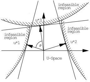
function) of the standard normal distribution. The MPP corresponds directly to the required reliability indexβ. The described approach represents the FORM method which is based on a linear approximation of the constraint function (refer to Fig. [3]).

u*1 _u*2

U−Space u*3

ρ

infeasible infeasible

region _region

Fig. 1. FORM procedure with linear approximation at the MPP. The third constraint does not influence the feasible area.

u*2 u*1

u*3

U−Space ρ infeasible

infeasible region

region

region infeasible

Fig. 2. The third constraint bounds the feasible area.

Importantly, the above procedure estimates the failure probability only for one constraint. In most optimization problems, the feasible area is bounded by more than one constraint and consists of constraint intersections. The fluc-tuation of the solution can be in any direction and so it is important to include all constraints in the reliability approximation. Simple bounds for the failure probability are given elsewhere [19],

maxIi=1Pi≤PF≤ I

i=1

Pi. (7)

Much closer bounds on the failure probability are given by Dietlevsen [1] which computes the joint failure probabilities of all constraints:

P1+

k

i=1

max ⎧ ⎨ ⎩Pi−

i−1

j=1

Pij,0

⎫ ⎬ ⎭≤PF

≤ k

i=1

Pi− k

i=2

maxj≤iPij.

(8) The formula depends on the sequence of the failure modes and a different order may cause different reliabilities. It is a practical experience that a good ordering is obtained by ordering the failure modes according to decreasing values Pi[14]. The joint probabilityPijis given by the CDF of the

bivariate normal distribution with

Pij= Φ(−βi,−βj, ρij) (9)

and the correlation coefficientρij is given by

ρij =cos u ∗ i,u∗j

u∗iu∗j

. (10)

Here, thecos(.)of the angle between twou∗ vectors. By using higher-order intersections it is possible to improve the bounds but this involves much more numerical effort with a little gain in accuracy of the result [15]. Summing up the ideas, we can replace the stochastic constraint in (1) for a single constraint by the following expression:

Pi≥R. (11)

If we include all constraints and measure PF with the

Ditlevson bounds then we get

1−

_k

i=1

Pi− k

i=2

maxj≤iPij

≥R. (12)

B. Methods For Finding the MPP

The search for the MPP point with a suitable algorithm is the computationally most expensive part of the FORM procedure. This is in itself an optimization problem [4]. Various methods have been proposed and an overview is given by Eldred [5]. For our following approach, we need the distance from the origin to the constraint in theU space. For this reason, we use the Reliability Index Approach (RIA) even if this procedure may be slower than others.

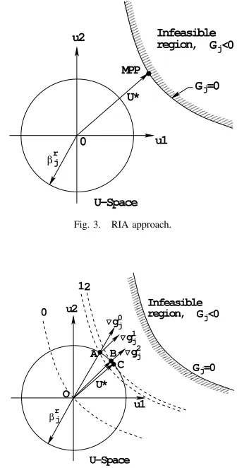
In the RIA approach, the MPP is found by searching for the point on the constraint boundary which has the minimal distance to the origin in theU space (see Fig. 3). This leads to the following minimization problem:

Minimize u

Subject to Gi(u) = 0. (13)

If we apply this optimization problem to every constraint, we get a vectoru∗, whereu∗_i=βiis the shortest distance

from the origin to the constrainti.

To solve the above problem, we use a fast gradient-based approximate approach proposed in [10], [4]. Fig. 4 illustrates the procedure and the steps are shown below.

Step 1 compute the gradient ∇g0i of constraintiat the

origin of the U space,

Step 2find the intersection (point A) of∇g0i and a circle

with radiusβi= 1,

Step 3compute the new gradient∇g1i at point A, Step 4find the intersection of∇gi1and the circle of radius

βi(point B),

Step 5 repeat step 3 and 4 until∇gii−∇gii+1 ≤

0,001. Then getu∗

Step 6perform a unidirectional search alongu∗ with the Newton Raphson approach until tolerance level= 0,001is met.

The convergence of this method is usually quick requiring only a derivate of the constraint in the U space. Since it is a gradient based procedure, there is no guarantee for convergence especially if highly non-linear constraints are involved. However, for most problems this approximation is sufficient and can be used.

G =0

βj r

G <0

U−Space u1 u2

0

Infeasible region,

MPP

U* j

j

Fig. 3. RIA approach.

G <0

βrj

gj0

G =0j

U−Space

Infeasible region, _j g_j1

0 1

u1 u2

O

A B C U*

g_j2

2

III. PROPOSEDACTIVECONSTRAINTAPPROACH In the FORM analysis, the integral in (4) is bound by the set of tangent hyperplanes at the MPP for the different con-straints (see Fig. 1). Normally, one calculates all the MPPs, then the correlation matrix and the probability matrix. The function for the reliability can be expressed asR(g1, ..., gI)

and depends on the distance from the constraints to the origin and the position of the different constraints relative to each other. Assume that there are three parallel constraints with different distances to the origin. Then only the closest constraint should be taken into account forPF as the others

do not increase PF. Fig. 2 shows an example in which

the feasible area is completely bound by three constraints. When the solution is moving away from constraint three, constraint three is no longer part of the bound and has no influence on the failure probability. If we know that constraint j does not biasPF, we could reduce the reliability function

toR(g1, . . . , gj−1, gj+1, . . . , gI). This means the inner loop

optimization for finding the MPP is not necessary and also the probability matrix can be reduced. Given the probability matrix

Pij =

⎛ ⎜ ⎜ ⎜ ⎜ ⎜ ⎝

P11

P12 P22

P13 P23 P33

..

. . ..

P1j P2j P3j · · · Pij

⎞ ⎟ ⎟ ⎟ ⎟ ⎟ ⎠

calculated using (9) and (6) the probability of violating constraintiis given byPiand also the failure probability for

the intersection of two constraints, given byPij. The upper

bound of (8) is

k

i=1

Pi− k

i=2

maxj≤iPij. (14)

Ifmaxj≤i(Pji)≥Pi, then no additional failure probability

is added. Given the above equation only a constraint parallel to another can get inactive. But also if they are not exactly parallel they are inactive because the intersection does only add irreducible failure probability. Therefore, we define the following:

Definition 1: Constraintiis called an inactive constraint, when the following criteria is fulfilled.

Pii≤maxj<iPji−∀ j < i ∈ J, (15)

wheredescribes the negligible failure probability. We have chosen = 0,0000009 for all our test cases. The impact of this approximation is much smaller than the influence of FORM and will not cause a loss in accuracy. The simulation results on test problems in this study also verify this. As an example, consider the following probability

matrix: ⎛

⎝ 0₀._.040_{005 0.020} 0.005 0.010 0.010

⎞ ⎠

Then the upper bound of the failure probability is(0.040− 0) + (0.020−0.005) + (0.010−0.010)or0.055. The third

constraint does not add any failure probability toPF because

its intersection with the second constraint is to large. If we calculate the reliability of that specific point again without considering the third constraint the result would be exactly the same.

Based on the above active constraint strategy, we suggest solving two types of problems: (i) finding multiple reliability solutions for a single-objective optimization problem and (ii) finding multiple Pareto-optimal solutions for a specified reliability value.

IV. FINDINGMULTIPLERELIABILITYSOLUTIONS We suggest a reliability-based optimization procedure based on evolutionary algorithms for finding solutions with respect to different reliability values simultaneously [10]. It was shown in the previous study that by introducing an additional objective of maximizing reliability(R or β) and treating the problem as a two-objective optimization problem (the other objective being the optimization of the original problem), the set of Pareto-optimal solutions consists of solutions corresponding to different reliability values. By analyzing these solutions, the user can also learn about how the solutions change with different reliability requirement and this knowledge may provide a plethora of important in-formation about the problem. This changes our optimization problem to the following problem:

Minimize μf(μX,d, μP),

Maximize R(μX,d, μP) =R= (1−PF),

Subject to hk(d)≥0, k= 1,2, ..., K,

β(L)≤β≤β(U), X(L)≤μX≤X(U),

d(L)≤d≤d(U).

(16)

To handle the reliability constraint, we use the RIA approach explained above as an inner-loop optimization. We then calculatePF with the Ditlevson bounds.

In real-world optimization problems there is often a large number of constraints. Since it is not known which constraints are active before finding the MPP, the above mentioned optimization problem has to be solved for every constraint. This becomes an expensive proposition. But in most situations, only a few constraints are active at the final solution. Thus, the active constraint strategy described above becomes a inexpensive procedure for computing failure prob-ability.

It is also intuitive that for a solution in a specific neigh-borhood involving a particular constraint set are active. Here, we use a book-keeping strategy in which the hierarchy of active constraints for each solution is stored. For evaluating a subsequent solution, a stored solution is first searched. If found, only the corresponding active constraints are consid-ered. If a subsequent solution happens to lie in a region deep inside the infeasible region, then only the most violated constraint of that area is evaluated. For solutions which do

not belong to a neighborhood, all constraints are evaluated. We present the complete constraint handling method in the following:

inputx

find closest pointmi toxin the memory

ifx−mi ≤then

if the stored reliability Pmi

F is smaller than parameter

kthen return Pmi

F else

calculate the MPP for the active constraints ofmi

calculatePFx with active constraints return PFx

end if else

evaluate MPP for all constraints identify the active constraints calculatePFx

storexandPFx return PFx end if

A. Simulation Results

To verify the suggested procedures, we apply them to two optimization problems: a two-variable test problem and a car side-impact problem.

Most classical reliability based methods start with search-ing for the deterministic solution. From this point the solution is shifted into the feasible area to satisfy the reliability constraint. With this method it is not secured that the obtained solution is the global optimum to the reliability based problem [10].

1) Two-Variable Multi-Modal Test Problem:Here we con-sider the following problem , the constraints are taken from [8]:

Minimize sin(3x2) + sin(3y2) +x+y, Maximize R(gi(x, y)) = (1−PF),

Subject to g1(x, y)≡ ₂₀1x2y−1≥0,

g2(x, y)≡ ₃₀1(x+y−5)2+₁₂₀1 +

(x−y−12)2_−1≥0,

g3(x, y)≡ _{x2+ 8}80_{y+ 5}−1≥0,

0≤x, y≤10.

(17)

To find the optimal solutions, we apply the NSGA-II with a population size of 100 for 200 generations. We restrict the reliability level to0.5≤ β ≤ 5.0 causing a reliability between 69.14625% and 99.99997%. The standard deviation of both variables is assumed to be 0.03. The objective functions, shown in Fig. 5, includes many local optima. It is interesting to note that as the reliability requirement increase,

the solutions tend to move away further from the constraint boundaries, thereby causing the basin of attraction to change from one local optimum to another. Every gap represents a change towards an inferior local optimum to satisfy the reliability requirement.

local optima 3 4

5 6 7 8 9

2.7 2.8 2.9 ₃

3.1 3.2 3.3 3.6 3.5 3.4

3.3 3.2 3.1

10

sin(x*x*3)+sin(y*y*3)+x+y

Fig. 5. Contour of the objective landscape of the test problem with four local optima.

function value with consideration of one constraint

with Ditlevson bounds

re

li

a

bilit

y

4 4.5 5 5.5 6 6.5 7 3.5

5 4.5 4 3.5 3 2.5 2 1.5 1 0.5

Fig. 6. Simulation results on the multi-modal test problem.

TABLE I

COMPARISON OF THE NUMBER OFMPPEVALUATIONS.

Method Car Side-Impact Proposed method 329.825 Without memory 1000.000

is defined as follows [10]:

Minimize (x1,...,x7)

f(x) =Weight,

Subject to c1(x)≡Abdomen load≤1kN, c2(x)≡V∗Cu≤0.32m/s, c3(x)≡V∗Cm≤0.32m/s,

c4(x)≡V∗Cl≤0.32m/s,

c5(x)≡Dur upper rib deflection≤32mm, c6(x)≡Dmrmiddle rib deflection≤32mm, c7(x)≡Dlrlower rib deflection≤32mm, c8(x)≡FPubic force≤4kN,

c9(x)≡Vel. of V-Pillar at mid. pt.≤9.9mm/ms, c10(x)≡Vel. of front door at V-Pillar≤15.7mm/ms,

0.5≤x1≤1.5, 0.45≤x2≤1.35,

0.5≤x3≤1.5, 0.5≤x4≤1.5,

0.875≤x5≤2.625, 0.4≤x6≤1.2,

0.4≤x7≤1.2.

(18)

There are 11 design variables, all related to the dimensions of a specific area in a car. The set can be divided intox= (x1, . . . , x7)for design variables andp= (p8, . . . , p11)for

uncertain parameters.

var

i

a

bl

es

weight

x1 _x3

x7 x5

x6 x4

x2

0.4 0.6 0.8 1 1.2 1.4 1.6

24 24.5 25 25.5 26 26.5 27 27.5 28 28.5 29 29.5

Fig. 7. Impact of the weight on the variables.

reliability x7

x3 x1

x5 x6 x2 x4

var

i

a

bl

es

0.4 0.6 0.8 1 1.2 1.4 1.6

3 2.5 2 1.5 1 z0.5

Fig. 8. Impact of the reliability on the variables.

Table II shows the angle between the constraints. The order of importance of the constraints depends on the chosen solutions and its distance to constraints. Every solution has its own order, although the order of constraints may be the

TABLE II

CORRELATION MATRIX WITH ANGLEρ.

c8 c2 c3 c7 c9 c10 c4 c5 c1 c6

c8 0 148 158 154 156 113 157 141 134 127 c2 148 0 14 26 10 67 18 34 24 49 c3 158 14 0 19 6 65 7 30 28 47 c7 154 26 19 0 19 65 25 37 33 54 c9 156 10 6 19 0 65 12 31 27 48 c10 113 67 65 65 65 0 66 94 68 110 c4 157 18 7 25 12 66 0 29 32 45 c5 141 34 30 37 31 94 29 0 44 19 c1 134 24 28 33 27 68 32 44 0 57

c6 127 49 47 54 48 110 45 19 57 0

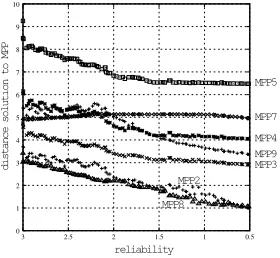
same for many solutions. In Fig. 9 we show the distance from the solution to the MPP. Constraint c2 and c8 are

reliability

di

s

t

ance so

l

u

ti

on

t

o

MPP

MPP8 MPP2

MPP3 MPP5

MPP9 MPP4 MPP7

0 1 2 3 4 5 6 7 8 9 10

3 2.5 2 1.5 1 0.5

Fig. 9. Distance from the solution to the MPP.

close throughout the reliability spectrum. That means the solution gets centered between these two constraints and if one constraint gets closer to a solution than the others gets farther. This is to conform with the correlation matrix (shown in Table II) which shows an angle of 148 degrees between these two constraints. Thus, the displacement of the Pareto-optimal front into the feasible area gets comprehensible. For constraintsc2 andc9, it is another interplay. The angle

between them is only 10 degrees, meaning that they are almost parallel and hence the one away from a solution does not have much effect on the reliability measure.

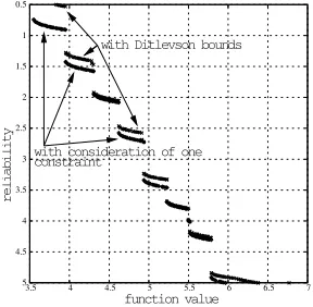
Fig. 10 shows the Pareto-optimal front obtained using three methodologies: (i) an earlier proposed one critical constraint approach which ignored all other constraints, (ii) our approach with Ditlevson bounds but all constraints are considered and (iii)our active constraint strategy in which only a few active constraints are considered. We restrictedβ to be between 0,5 (reliability of 69.14625%) and 3 (reliability of 99.865%). Like in the case of two-variable test problem shown earlier, the Pareto-optimal front using our approaches move deeper insider the search space due to a tighter computation of reliability. The earlier approach [10] used an optimistic reliability computation thereby resulting in an ap-parently better Pareto-optimal front. Interestingly, there is no

constraint consideration of one

consideration of active constraints

consideration of all constraints

weight

re

li

a

bilit

y

23 24 25 26 27 28 29 30

0.5

1

1.5

2

2.5

3

Fig. 10. Comparison between the proposed method where only active constraints are evaluated, where all constraints are evaluated, and where only one critical constraint is evaluated.

difference between the Pareto-optimal fronts obtained using both our approaches. However, our active constraint strategy requires only 32% of the total constraint calls compared to the all-constraint approach (refer to Table I). It is clear from Fig. 9 that only two constraints are critical in most reliable solutions. Thus, the active constraint strategy, in this problem, becomes very efficient in reducing the computational effort yet producing almost an identical accuracy in the result compared to the expensive all-constraint strategy.

V. MULTI-OBJECTIVEOPTIMIZATION FOR ASPECIFIED RELIABILITY

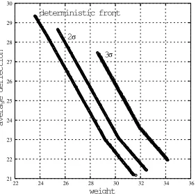
These problems are multi-objective in nature, but instead of finding the deterministic Pareto-optimal front, here our interest is to find a reliable front for a specified reliability. We use the active constraint strategy along with the RIA approach. If at a point, the computed reliability is smaller than the specified reliability, we declare the solution as an infeasible one. NSGA-II is employed for finding the reliable frontier. We illustrate the working of this procedure by solving a two-objective version of the car side-impact problem.

A. Two-Objective Car Side-Impact Problem

We use an additional objective of minimizing the average rib deflection, calculated by taking the average of three deflections g5(x), g6(x), g7(x). Figure 11 shows the

re-liable frontier for different reliability values using Ditlevson bounds (i) on all constraints and (ii) on active constraints only. Interestingly, for each specified reliability value, both all-constraint and active-constraint strategies have found an identical Pareto-optimal frontier. This usually happens when inactive constraints are far away from the optimal solutions. To investigate the distance of constraints from the optimal solution at different Pareto-optimal solutions, we plot the distance versus the weight objective at the solutions in Fig. 12. It is clear that only one constraint (the Pubic force constraint c8) is active and critical for all Pareto-optimal

solutions in this problem. For better deflection solutions, the other constraints are more away from this constraint, thereby causing a negligible contribution in the computation of the

2σ

3σ

average

d

e

fl

ect

i

on

weight deterministic front

21 22 23 24 25 26 27 28 29 30

22 24 26 28 30 32 34 36

Fig. 11. Two-objective Pareto-optimal fronts for different specified relia-bilities.

weight

di

s

t

ance so

l

u

ti

on

t

o

MPP MPP9

MPP8 MPP2

MPP3

MPP7 MPP4

MPP5

0 2 4 6 8 10 12 14

25 26 27 28 29 30 31 32 33

Fig. 12. Only one constraint affects the solution in a significant manner.

reliability of these solutions. Thus, both all-constraint and active-constraint strategies perform more or less the same. Also, identical reliable frontiers were obtained in the earlier study using the single critical constraint strategy [10] for the identical reason of having one critical constraint for each solution in this problem.

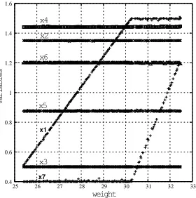
To investigate the properties of decision variables common to obtained Pareto-optimal solutions for a particular reliabil-ity (forβ= 2), we plot all seven variables against the weight objective in Fig. 13. Interestingly, six variables remains fixed in all solutions and for smaller weight solutions, a change in variable x1 changes one Pareto-optimal solution from

another, while for smaller deflection solutions, a change in x7 changes one Pareto-optimal solution from another.

Interestingly, with an increase in x1 the weight increases

at the benefit of smaller deflection but when x1 reaches its

upper limit, it cannot increase any further. To still make a trade-off between weight and deflection, the next thing to do is to increasex7to obtain a better deflection solution. Such

weight x4

x6 x2

x5

x3 x1

x7

var

i

a

bl

es

0.4 0.6 0.8 1 1.2 1.4 1.6

25 26 27 28 29 30 31 32 33 ’x5.txt’

Fig. 13. Here the variables withβ = 2are plotted against the weight (deflection problem).

VI. CONCLUSIONS

In this paper, we have extended the one-critical constraint strategy adopted in an earlier study for finding reliable frontiers for handling uncertainties in decision variables and parameters. Based on Ditlevsen’s probability computation, we have suggested two approaches: based on a composite success probability computation: (i) using all constraints and (ii) using only active constraints. On two types of multi-objective optimization problems involving test problems and a car side-impact design problem, we have shown that our proposed approaches produce a more accurate reliability estimate than the previous one-critical constraint strategy. Moreover, both of our approaches produce more or less identical frontiers, except that the active constraint strategy is computationally cheaper than the all-constraint strategy. Based on all these comparative studies, we recommend fur-ther and immediate use of active constraint strategy to more complex robust and reliability-based optimization problems.

ACKNOWLEDGMENT

The authors would like to thank Mr. Sulabh Gupta for his help.

REFERENCES

[1] AO. Ditlevsen,Narrow reliability bounds for structural system, J. Struct. Mech. 4 (1) 431-439, 1979.

[2] M. Rosenblatt, Remarks on a multivariate transformation, Ann Math.Stat., 23 470-472, 1952.

[3] AM. Hasofer, NC. Lind,An exact and invariant first order reliability format, J Eng Mech Div ASCE, 100(EM1):111 ˝U21, 1974.

[4] X. Du, W. Chen,A Most Probable Point Based Method for Uncertainty Analysis, Journal of Design and Manufacturing Automation, 1, pp. 47-66, 2001.

[5] M. S. Eldred, B. J. Bichonz, B. M. Adamsx,Overview of Reliability Analysis and Design Capabilities in DAKOTA, Conference Paper, NSF Workshop on Reliable Engineering Computing (REC 2006), Savannah, GA, February 2006.

[6] K. Deb, Multi-objective optimization using evolutionary algorithms, Chichester, UK: Wiley, 2001.

[7] H. Agarwal,Reliability based design optimization: Formulations and Methodologies, PhD thesis, University of Notre Dame, 2004. [8] L. Gu, R. J. Yang, C. H. Tho, L. Makowski, O. Faruque, and Y.

Li, Optimization and robustness for crashworthiness of side impact, International Journal of Vehicle Design, 26(4), 2001.

[9] K. Deb, S. Agrawal, A. Pratap, and T. Meyarivan,A fast and elitist multi-objective genetic algorithm: NSGA-II, IEEE Transactions on Evolutionary Computation, 6(2):182-197, 2002.

[10] K. Deb, D. Padmanabhan, S. Gupta, A. K. and Mall, Handling Uncertainties Through Reliability-Based Optimization Using Evolu-tionary Algorithms, Fourth International Conference on Evolutionary Multi-Criterion Optimization (EMO 2007) pp. 66-88 Lecture Notes on Computer Science 4403, 2007.

[11] O. Ditlevsen, H. O. Madsen,Structural Reliability Methods, New York: Wiley, 1996.

[12] HO. Madsen, S. Krenk, NC. Lind, Methods of structural safety, Englewood Cliffs (NJ): Prentice-Hall, Inc., 1986.

[13] R. Rackwitz,Reliability analysis ˚U A review and some perspectives, Structural Safety 23(4):365 ˝U 95, 2001.

[14] C.A. Cornell,Bounds on the reliability of structural systems, J. Struct. Div., ASCE, 93 (ST1) 171-200, 1967.

[15] K. Ramachandran, M. BakerNew reliability bound for series systems, In: Konishi I, Ang AH-S, Shinozuka M, editors. Proc. ICOSSAR Š85, Kobe; p. 157 ˝U169 [Vol. I], 1985

[16] J. H. Holland,Adaptation in Natural and Artifcial Systems, Ann Arbor, MI: MIT Press, 1975.

[17] D. E. Goldberg,Genetic Algorithms for Search, Optimization, and Machine Learning, Reading, MA: Addison-Wesley, 1989.

[18] K. Deb, A. Srinivasan Innovization: Innovating design principles through optimizationProc. of the Genetic and Evolutionary Computation Conference (GECCO-2006), New York: The ACM Press, p. 1629–1636, 2006

[19] Henrik O. MadsenFirst Order vs. Second Order Reliability Analysis of Series StructuresStructural Safety, 2 207-214, 1985

APPENDIX

f(x) = 1.98 + 4.9x1+ 6.67x2+ 6.98x3+ 4.01x4+ 1.78x5 +0.00001x6+ 2.73x7,

g1(x) = 1.16−0.3717x2x4−0.00931x2x10−0.484x3x9 +0.01343x6x10,

g2(x) = 0.261−0.0159x1x2−0.188x1x8−0.019x2x7 +0.0144x3x5+ 0.87570.001x5x10+ 0.08045x6x9 +0.00139x8x11+ 1.575(10−6)x10x11,

g3(x) = 0.214 + 0.00817x5−0.131x1x8−0.0704x1x9 +0.03099x2x6−0.018x2x7+ 0.0208x3x8+ 0.121x3x9 −0.00364x5x6+ 0.0007715x5x10−0.0005354x6x10 +0.00121x8x11+ 0.00184x9x10−0.018x2x2,

g4(x) = 0.74−0.61x2−0.163x3x8+ 0.001232x3x10 −0.166x7x9+ 0.227x2x2,

g5(x) = 28.98 + 3.818x3−4.2x1x2+ 0.0207x5x10 +6.63x6x9−7.77x7x8+ 0.32x9x10,

g6(x) = 33.86 + 2.95x3+ 0.1792x10−5.057x1x2−11x2x8 −0.0215x5x10−9.98x7x8+ 22x8x9,

g7(x) = 46.36−9.9x2−12.9x1x8+ 0.1107x3x10,

g8(x) = 4.72−0.5x4−0.19x2x3−0.0122x4x10 +0.009325x6x10+ 0.000191x11x11,

g9(x) = 10.58−0.674x1x2−1.95x2x8+ 0.02054x3x10 −0.0198x4x10+ 0.028x6x10,

g10(x) = 16.45−0.489x3x7−0.843x5x6+ 0.0432x9x10 −0.0556x9x11−0.000786x11x11.