Bayesian Processor of Output for Probabilistic Quantitative Precipitation Forecast over Central and West Africa

(1)

ISSN Online: 2160-0422 ISSN Print: 2160-0414

Bayesian Processor of Output for Probabilistic

Quantitative Precipitation Forecast over

Central and West Africa

Romeo S. Tanessong

1,2*

, Derbetini A. Vondou

2

, P. Moudi Igri

2

, F. Mkankam Kamga

2

1_{School of Wood, Water and Natural Resources, Faculty of Agronomy and Agricultural Sciences, University of Dschang,} Dschang, Cameroon

2_{Laboratory for Environmental Modelling and Atmospheric Physics, Department of Physics, University of Yaounde 1,} Yaounde, Cameroon

Abstract

The main goal of this work is a feasibility study for the Bayesian Processor of Output (BPO) method applied to tropical convective precipitation regimes over Central and West Africa. The study uses outputs from the Weather Re-search and Forecasting (WRF) model to develop and test the BPO technique. The model ran from June 01 to September 30 of 2010 and 2011. The BPO method is applied in each grid point and then in each climatic zone. Prior (climatic) distribution function is estimated from the Tropical Rainfall Mea-suring Mission (TRMM) data for the period 2002-2011. Many distribution functions have been tested for the fitting. Weibull distribution is found to be a suitable fitting function as shown by goodness of fit (gof) test in both cases. The rain pattern increases with the value of the probability p. BPO method noticeably improves the distribution of precipitation as shown by the spatial correlation coefficients. It better detects certain observed maxima compared to the raw WRF outputs. Posterior distribution (forecasting) functions allow for a simulated rainfall amount, to deduce the probability that observed rain-fall rain-falls above a given threshold. The probability of observing rainrain-fall above a given threshold increases with simulated rainfall amounts.

Keywords

Probabilistic Quantitative Precipitation Forecast, BPO, WRF, Weibull Distribution

1. Introduction

Economies of sub-Saharan Africa largely depend on agriculture. The agriculture How to cite this paper: Tanessong, R.S.,

Vondou, D.A., Igri, P.M. and Kamga, F.M. (2017) Bayesian Processor of Output for Prob-abilistic Quantitative Precipitation Forecast over Central and West Africa. Atmospheric and Climate Sciences, 7, 263- 286. http://dx.doi.org/10.4236/acs.2017.73019

Received: March 9, 2017 Accepted: July 1, 2017 Published: July 4, 2017

http://creativecommons.org/licenses/by-nc/4.0/

(2)

is essentially rain-fed. Precipitation is the most important and most widely stu-died weather variable ([1] [2] [3] [4] [5]). Important decisions in agriculture, hydrology, aviation, event planning and other areas depend on the presence or absence of precipitation, as well as precipitation accumulation. Reliable predic-tions of precipitation occurrence and precipitation amount are useful for above mentioned applications.

For these reasons, there is a great deal of research activities to improve quan-titative precipitation forecast (QPF) and weather centers continuously evaluate their operational high-resolution limited-area models to trace error sources. QPF is particularly challenging over Equatorial Africa, especially capturing small convective cells that constitute most of the rain events ([6][7][8]).

Furthermore, QPFs obtained from a single numerical weather prediction (NWP) model are deterministic, and thus do not convey any information about the uncertainty about the prediction, which is a shortcoming in weather-related decision-making [9]. One approach to incorporating uncertainty information into weather forecasting is via ensembles of numerical forecasts ([10] [11]). While this is a major advance, the use of statistical post processing techniques for numerical forecasts remains essential. Several methods have been developed to statistically post process numerical predictions of precipitation occurrence and produce probabilistic quantitative precipitation forecasts. They include li-near regression ([12] [13][14]), quantile regression ([15][16]), logistic regres-sion ([17] [18]), neural networks ([19] [20]), binning techniques ([21] [22]), hierarchical models based on climatic prior distributions [23], and two-stage models in which a Gamma density is employed to model precipitation accumu-lation ([24][25][26][27]).

In this paper, Bayesian Processor of Output for probabilistic quantitative pre-cipitation forecasts is used. The Bayesian Processor of Output (BPO) is a theo-retically-based technique for probabilistic forecasting of weather variates. It processes output from a numerical weather prediction (NWP) model and opti-mally fuses it with climatic data in order to quantify uncertainty about a predic-tand. The theoretical structures of the BPO are derived from the laws of proba-bility theory.

As is well known, Bayes theorem provides the optimal theoretical framework for fusing information from different sources and for obtaining the probability distribution of a predictand, conditional on a realization of predictors, or condi-tional on an ensemble of realizations [28].

(3)

2. Model Description and Experimental Design

2.1. Model Description

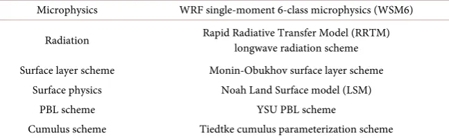
We performed simulations using version 3.3 of the Advanced Research Weather Research and Forecasting (ARW-WRF) model [29], which is being developed by the Mesoscale and Meteorology Division of the National Center for Atmospheric Research (NCAR). The WRF model is a numerical weather prediction model de-signed for a wide range of applications, ranging from idealized research to oper-ational forecasting. It is a fully compressible, Euler nonhydrostatic model, with mass-based, terrain-following hydrostatic pressure vertical coordinates and Arakawa C-grid horizontal staggering. For the current work we choose the third-order Runge-Kutta split-explicit time-integration scheme and sixth-order centered differencing for advection and prognostic variables, conserving the flux form of mass, momentum, entropy, and scalars. Previous work has been done (not shown here) to determined satisfactory configurations by testing numerous physical parameterizations. Satisfactory Physical configurations are summarized

in Table 1.

Hong et al. [30] developed the single-moment six-class microphysics scheme for the WRF, which includes graupel as an additional predictive variable. This microphysics scheme was found to significantly influence the evolution of sur-face precipitation [30]. Also used is the rapid radiative transfert model (RRTM)

[image:3.595.208.532.634.734.2]

[31]. The RRTM longwave scheme accounts for multiple bands, trace gases, and microphysics species. The first-order closure scheme of Yonsei University (YSU) used for the planetary boundary layer (PBL) is a non-local K scheme with an ex-plicit entrainment layer and parabolic K profile in the unstable mixed layer. The Noah land surface model (Noah LSM) is used to calculate soil temperature and moisture. The Tiedtke convection scheme is a bulk flux convection scheme [32]. It handles three types of convection: deep, middle level, and shallow convection. In the Tiedtke scheme, only one convective cloud is considered, comprising one single saturated updraft. Entrainment and detrainment between the cloud and the environment can take place at any level between the free convection level and the zero-buoyancy level. There is also one single downdraft extending from the free sinking level to the cloud base. The mass flux at the top of the downdraft is a constant fraction of the convective mass flux at the cloud base. This down-draft is assumed to be saturated and is kept at saturation by evaporating precipi-tation. The original closure assumption for deep convection relies on a closure in

Table 1. Physics parameterizations used in the experiments.

Microphysics WRF single-moment 6-class microphysics (WSM6)

Radiation Rapid Radiative Transfer Model (RRTM) _{longwave radiation scheme}

Surface layer scheme Monin-Obukhov surface layer scheme

Surface physics Noah Land Surface model (LSM)

PBL scheme YSU PBL scheme

(4)

moisture convergence, while that used in this version is based on the convective available potential energy (CAPE) modified by [33].

2.2. Experimental Setup

The model is run from June 01 to September 30 of 2010 and 2011. The initial and boundary conditions are provided by the National Center for Environmen-tal Prediction (NCEP) Global Forecasting System (GFS) three hourly products. We use the 0000 UTC cycle and run the WRF model for 48 hours starting at 0000 UTC. The model is set at a horizontal grid resolution of 25 km × 25 km and has 41 vertical levels. Data analysed are total precipitation amount for the 24-hourperiod starting at 0600 UTC, thus having 6 hours of spinup (from 00 UTC to 0600 UTC).

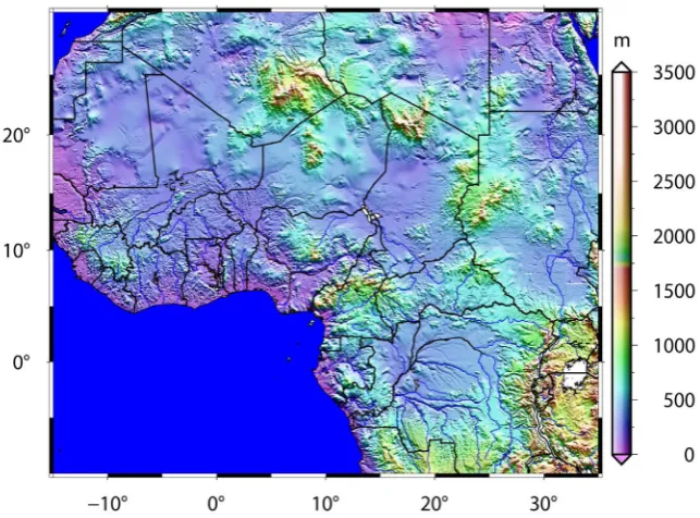
2.3. Area of Study

The study area extends from 15˚W to 30˚E and 10˚S to 30˚N (Figure 1). A re-gionalization of the domain was carried out using the one-degree daily precipi-tation data set developed by the Global Precipiprecipi-tation Climatology Project (GPCP) [34] for the period 1997-2008.

Six distinct main climatic regions (Figure 2) were delineated using a Ward’s clustering technique ([35][36][37][38][39]). In the following, the analysis will be conducted in each of the five regions (Region 2 to Region 6) that cover the study area (See Figure 2).

[image:4.595.214.536.477.715.2]

Region 2 covers arid (Sahara Desert) and semiarid (Sahel) zones over Mauri-tania, Mali, Niger, Chad and parts of Sudan, Cameroon and Nigeria. In the northern part of this region the climate is uniformly dry, with most areas re-ceiving less than 130 mm/year of rain, some getting none at all for some years.

(5)

[image:5.595.219.528.66.230.2]

Figure 2. Homogeneous rainfall regions for the June-September (JJAS) season.

The southern part serves as a transition zone between the arid Sahara and the wetter savanna region further south. Annual rainfall averages between 100 and 200 mm received from June to September (Figure 3). Region 3 covers Liberia, Ivory Coast, Ghana, Togo, Benin, Nigeria, Cameroon and Central African Re-public, in the area bordering the Gulf of Guinea. It has both areas of hot dry season (moderate rainfall) and wet climate (high, all-year rainfall). Rainfall ranges between 100 and 400 mm/year in the former and as much as 1800 mm in the latter. Region 4 represents the transition between the ocean and the conti-nent. Breeze phenomena are very recurrent. Region 5 covers the South Atlantic Ocean and represents an oceanic climate. Region 6 is characterized by the tropi-cal wet climate.

2.4. Data Sources and Structure

2.4.1. TRMM 3B42

For the purpose of verification we used Tropical Rainfall Measuring Mission (TRMM) data as ground truth. TRMM data show that the JJAS seasons 2010 and 2011 were wet and dry respectively (Figure 4). TRMM was used instead of gauge data because of the irregular spatial distribution of gauges and the sparse net-work in the region. TRMM is a joint mission of the American National Aero-nautics and Space Administration (NASA) and the Japanese National Space De-velopment Agency (NASDA) to measure precipitation in the tropics and sub-tropics. In this work, version 6 of the 3B42 data set is used. It provides three hourly estimations of rainfall on a 0.25˚ × 0.25˚ grid. These data are provided online by the NASA at http://mirador.gsfc.nasa.gov. Nicholson et al. [40] eva-luated TRMM products over West Africa over the May to September season. They found that TRMM-merged rainfall products showed excellent agreement with gauge data.

Although the 0.25˚ grid spacing of TRMM data is close to WRF’s 25 km, they were regridded in order to achieve coincidence of both grids points.

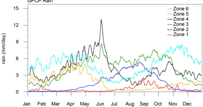
2.4.2. 1DD GPCP Precipitation Data

(6)

[image:6.595.211.540.78.251.2] [image:6.595.211.533.291.438.2]

Figure 3. Mean rainfall (mm) for the period 1997 to 2008.

Figure 4. Mean JJAS anomalies for years 2010 and 2011.

from Global precipitation Climatology Project. The GPCP algorithm combines precipitation estimates from several sources, including infrared (IR) and passive microwave (PM) rain estimates, and rain gauge observations [41]. The IR data come mainly from the different Geostationary Meteorological Satellites but also from polar-orbiting satellites for high latitudes [42]. The microwave data come from the Special Sensor Microwave Imager (SSM/I) onboard the Defense Me-teorological Satellite Program. The multi-satellite estimates are first adjusted to-wards the large-scale gauge average for each grid box, and then combined with gauge analysis using a weighted average. 1DD GPCP Precipitation data are used in the present work to subdivide the study area into subdomains and to deter-mine seasonal cycle in each.

3. Bayesian Processor of Output Techniques

(7)

probability of observing a rainfall amount greater than 10 mm, knowing that the forecast amount is 1 mm. The concept is illustrated in Figure 5. The BPO is operationalized by the meta-Gaussian model ([43][44][45]). It is described be-low in terms of input elements and forecasting equations.

3.1. Input Elements

The following algorithm deﬁnes the input elements, outlines the estimation procedure, and details the calculation of the posterior parameters (the para-meters of the forecasting equations).

Step 0: Given are two samples, the climatic sample of the predict and W, and the joint sample of the predictor vector and the predict and (X, W), re-spectively:

( )

{

w n :n=1,,M

}

,

( ) ( )

(

)

{

x n ,w n :n=1,,N

}

,

where x n

( )

=

(

x n1

( )

,,xI

( )

n

)

and N≤M ; all realizations of W from the joint sample are included in the climatic sample. The index I scans over the

number of predictors.

Step 1: Using the climatic sample, the prior (climatic) distribution function G of predict and W is estimated, such that G w

( )

=P W

(

≤w

)

; P denotes

the probability.

Let g denote the corresponding prior (climatic) density function of W. Step 2: Using the marginal sample

{

x n_i

( )

:n=1,,N

}

of the joint sample, we estimate the marginal distribution function Ki of predictor Xi, such that

( )

(

)

, 1, , .

i i i i

K x =P X ≤x i=  I

(The bar over Ki signifies that this is only an initial distribution function of Xi, which need not cohere to the specified prior distribution function of W and the yet-to-be-constructed family of likelihood functions. This detail is accounted for in the derivation of the meta-Gaussian BPO, and thus need not be considered in application.)

Step 3: The normal quantile transform (NQT) of the predictand and of every predictor is defined:

( )

(

)

1

,

V =Q− G W

( )

(

)

1

, 1, , ,

i i i

Z =Q− K X i=  I

(8)

where Q is the standard normal distribution function, and 1

Q− is the inverse

of Q. Next, we apply the NQT to each realization in the original joint sample; speciﬁcally, for n=1,,N, we calculate v n

( )

=Q−1

(

G w n

(

( )

)

,

( )

1

(

( )

)

, 1, ,

i i i

z n =Q− K x n i=  I; then the transformed joint sample is

eva-luated

{

(

z n v n

( ) ( )

,

)

:n=1,,N

}

, where z n

( )

=

(

z n₁

( )

,,z_I

( )

n

)

.

Step 4: Using the transformed joint sample, we estimate the following moments. For the transformed predictand V,

( )

2

( )

0 E V , 0 Var V

µ = σ = _.

For every transformed predictor Z ii, =1,,I ,

( )

2

,

i E Zi i Var Zi

µ = σ = _,

(

)

0 ,

i Cov Z Vi

σ = . For i=1,,I−1 and j= +i 1,,I, σij=Cov Z Z

(

i, j

)

. The estimates of variances and covariances should be the maximum like-lihood estimates (i.e., they should be calculated using N as the divisor).

Step 5: We form two I-dimensional column vectors µ=

(

µ1,,µI

)

,

(

10, , I0

)

σ= σ _σ , the transpose of vector σ, which is denoted σT, and an

I×I symmetric matrix Σ =

{ }

σ_ij , with 2 ii i

σ =σ _for i=1,,I, and

ji ij

σ =σ for i=1,,I−1 and j= +i 1,,I . Next we calculate an I×I

symmetric matrix

(

)

1

2 T

0

M = Σ −σ σσ− − (1)

Step 6: The values of the posterior parameters are calculated as follows:

1 4 ₂ 0 T 4 0 T M

σ

σ σ

 

=  ₊ 

  (2)

2

T T

2 0

T

c σ M

σ

= ₍₃₎

T 0

0 2

0

c c µ σ µ σ

 

=  − 

  (4)

where T

[

]

1, , I

c = c  c is an I-dimensional row vector.

3.2. Forecasting Equations

Given a prior distribution function G of predict and W and given a realiza-tion x=

(

x1,,xI

)

of the predictor vector, the meta-Gaussian posterior dis-tribution function of predict and W is specified by the equation

( )

1

(

( )

)

1

(

( )

)

0 1

1 I

i i i

i

w Q Q G w c Q K x c

T

− −

=

  

Φ = _ _ − − __

 



∑

 (5)

For any number p such that 0< <p 1, the p-probability posterior quantile of predict and W is specified by the equation

( )

(

)

( )

1 1 1

0 1

I

p i i i

i

w G− Q c Q− K x c TQ− p

=

  

= _ _ + + __

 



∑

 (6)

Given also a prior density function g of predict and W, the meta-Gaussian posterior density function of predict and W is specified by the equation

( )

1 1

{

₁

(

( )

)

2 ₁

(

( )

)

2

}

( )

exp

2

w Q G w Q w g w

T

φ

₌  _ − _ ₋_ − _Φ _ 

     

(9)

In the current work, one predictor is used. When there is only one predic-tor (I = 1), its subscript is omitted. Thus X replaces X₁, K replaces K₁,

and the forecasting Equations (5)-(6) can be written

( )

1

(

( )

)

1

(

( )

)

0 1

1 I

i i

w Q Q G w c Q K x c

T

− −

=

  

Φ = _ _ − − __

 



∑

 (8)

( )

(

)

( )

1 1 1

0 1

I

p i

i

w G− Q c Q− K x c TQ− p

=

  

= _ _ + + __

 



∑

 (9)

In the following, processing will be done by grid point and climatic zones.

4. Results

4.1. Processing by Grid Point

4.1.1. Prior Distribution Function

The prior distribution function G of precipitation amount W is conditional on precipitation occurrence: G w

( )

=P W

(

≤w W| >0

)

. It is estimated from the TRMM data for the period 2002-2011. This estimation is done at any grid point. Many distribution functions are tested for the fitting. Weibull distribution is found to be a suitable fitting function as shown by goodness of fit (gof) test (not shown here).

4.1.2. Marginal Distribution Function

The single predictor X is the estimate of the 24-h total precipitation. The mar-ginal distribution function K of X is conditional on precipitation

occur-rence:

( )

(

| 0

)

K x =P X ≤x W> . It is estimated for WRF model outputs cover the

period JJAS2010-2011 from the joint sample. Weibull distribution is also found to be more suitable.

4.1.3. Transformed Rain wp

Once the five elements

(

G K T c c, , , 0, 1

)

are specified, the transformed rain may be calculated, given any value p of the probability.

From the definition, the number p is the probability that the value of the pre-cipitation is less than or equal to w p. In this section, the number p is simply in-terpreted as the probability that the rain is equal to w p. Only values of p for which the spatial distribution of precipitation is close to the observations will be presented.

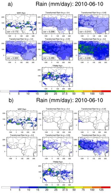
Figure 6(a) represents the weather of June 10, 2010. This figure shows that

the rain pattern produced by the BPO method is denser than those produced by WRF and TRMM for great values of the probability p. The algorithm used in the BPO method gives the cumulative distribution (CDF) of the rains. This is why the intensity of rainfall increases with the probability. Indeed, the chances of ob-serving the precipitation less than 5 mm at a point are less than the chances to observe precipitation less than 10 mm at this point. In the following, p will be simply taken as the probability that the rain patterns be that shown on the maps.

(10)

[image:10.595.167.538.68.710.2]

(11)

the field, compared to observations.

For p = 0.4 (Figure 6(a)), the maximum rainfall is located on the coast of Libe-ria, Sierra Leone and Guinea. The intensity of rainfall in the region is about 15 mm. The TRMM observations confirm that these areas were rainy at June 10, 2010.

The observed intensity is 25 mm instead of 15 mm as forecasted by the BPO method for p = 0.4. For p = 0.45, other maxima are found over West Cameroon and northern Burkina Faso. It is generally found that when the probability p in-creases, the areas that have the maxima are preserved with the difference that intensity also increases. For p = 0.6, some observed maxima are located by the BPO method. These include the maximum observed on the north of the Central African Republic and the south-eastern Nigeria.

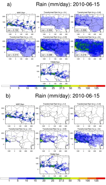
Figure 7(a) displays rainfall patterns of June 15, 2010. The field and intensity

of rainfall increase with the value of the probability p. Maxima are detected by the BPO method especially for p = 0.45, 0.5, 0.55 and 0.6. The maximum ob-served in southern Nigeria is well reproduced by the BPO method. Intensities are in the same order for p = 0.6. This intensity is about 50 mm. For the values of p less than 0.6, these areas of maximum intensity are well detected but the inten-sities are underestimated. The maxima observed on the coast of Liberia, Sierra Leone, the Guinea Conakry are detected by the BPO method. The TRMM ob-servations also show maxima rainfall in southern Central African Republic, northern Democratic Republic of Congo. These maxima were not well localized by BPO method.

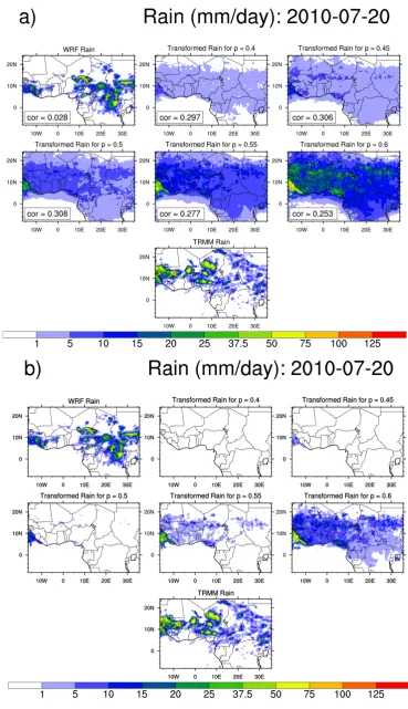
Figure 8(a) shows the rains patterns of 20-07-2010. The maximum observed

on the coast of Guinea Conakry is well locate for p = 0.6. Some maxima observed in southern Mali, south of Niger and central Nigeria have not been well detected by the BPO method.

Given the foregoing, it is found that BPO method introduced background noise. It provides low rainfall almost throughout the study area especially when the value of the probability p increases. This led us to subtract the average daily climatology (8.8 mm) over the entire region to get rid of this noise. Figure 6(b),

Figure 7(b) and Figure 8(b) show these new maps. Figure 6(b) shows the rains

patterns of 10-06-2010. This field is less dense than that of Figure 6(a). Some maxima are well captured by the BPO method. These maxima are observed on the coast of Sierra Leone, eastern Chad, the southwest coast of Cameroon and eastern Senegal. In general, withdrawal of the daily average climatology reduces the field of the rains. For some values of the probability (p = 0.55 and p = 0.6), this field is close enough observed field.

4.2. Processing by Climatic Zones

In the following, the analysis will be conducted in each of the five regions (Region 2 to Region 6) that cover the study area (see Figure 2). The following figures show prior and posterior distribution functions and prior and posterior densities.

4.2.1. Region 2

(12)

[image:12.595.169.538.69.712.2]

(13)

[image:13.595.165.535.70.712.2]

(14)

[image:14.595.237.507.76.568.2]

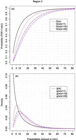
Figure 9. Examples of probabilistic forecasts of the precipitation amount W, conditional on precipitation occurrence, W greater than 0, and based on three different realizations x = 1, 10, 25 [mm] of predictor X for 24-h total precipitation amount output from the WRF model: (a) the prior (climatic) distribution function G and three posterior distribution func-tions G(w|x = 1), G(w|x = 10), G(w|x = 25); (b) the prior (climatic) den-sity function g and three posterior denden-sity functions g(w|x = 1), g(w|x = 10), g(w|x = 25).

(15)

any point in the Region 2 is 0.75. This means that there is 75% chance to observe at any point of this region an amount of rain less or equal to 20 mm. We deduce that the probability of observing rainfall amount greater than 20 mm is 0.25, that is there is only 25% chance to observe rain greater than 20 mm in intensities.

For simulated value of 10 mm of rainfall, the probability of observing rainfall less than or equal to 20 mm is 0.65. That is 65% chance to observe rainfall ≤20 mm when the model simulates 10 mm of precipitation at a point. We deduce from the above that the probability of observing rainfall greater than 20 mm is 0.35.

Thus, there is 35% chance of observing rainfall intensities greater than 20 mm at a point when the model simulates 10 mm of rainfall. For a simulated value of 25 mm, the probability of observing rainfall ≤ 20 mm is 0.58, that is there is 58% of chance of observing rainfall ≤ to 20 mm when the WRF model simulates 25 mm of rainfall at a point. The probability to observe rainfall intensity greater than 20 mm is 0.42; that is 42% of chance.

Based on the above analysis, it appears that the probability of observing rain-fall above a given threshold increases with simulated rainrain-fall amounts. This re-sult is consistent with that of Tanessong et al. [46].

Figure 9(b) represents the prior (climatic) density function g and three

post-erior density functions based on three different realizations of predictor X: 1 mm, 10 mm and 25 mm. For a simulated rainfall amount of 1 mm, the most likely rainfall value that can be observed is 5 mm. This most likely value is 8 mm when simulated rainfall amount is 10 mm and becomes 12 mm for a simulated rainfall amount of 25 mm. Thus, when the simulated rainfall amount increases, the chances of observing heavy rainfall also increase. These results thus streng-then those found previously. Figure 9(b) also shows that the density decreases as the observed quantities increase, indicating that heavy rainfall events are rare and therefore difficult to predict.

4.2.2. Region 3

Figure 10(a) represents the prior (climatic) distribution function G and three

posterior distributions functions based on three different realizations: 1 mm, 10 mm and 25 mm of predictor X. For simulated rainfall amount of 1 mm, the probability to observe rainfall ≤ 20 mm is 0.90, that is 90% of chances. Then the chances of observing the rainfall amounts greater than 20 mm are 10% only when simulated rainfall amount is 1 mm. For simulated rainfall amounts of 10 mm, the probability of observing rainfall ≤ 20 is 0.75 mm, for example; that is 75% chance.

Thus the probability of observing rainfall greater than 20 mm is 0.25; yielding 25% chance. For simulated rainfall amount of 25 mm, the probability of observ-ing rainfall ≤ 20 mm is 0.7; 70% chance. The chances of observobserv-ing the rainfall greater than 20 mm are 30%.

(16)

Figure 10. Examples of probabilistic forecasts of the precipitation amount W, conditional on precipitation occurrence, W greater than 0, and based on three different realizations x = 1, 10, 25 [mm] of predictor X for 24-h total precipitation amount output from the WRF model: (a) the prior (climatic) distribution function G and three posterior distribu-tion funcdistribu-tions G(w|x = 1), G(w|x = 10), G(w|x = 25); (b) the prior (cli-matic) density function g and three posterior density functions g(w|x = 1), g(w|x = 10), g(w|x = 25).

[image:16.595.236.509.79.556.2]

(17)

Figure 10(b) represents the prior (climatic) density function g and three posterior density functions. For the simulated rainfall amount of 1 mm, the most likely value that can be observed is 4 mm with a density of 0.06. The most likely value is 7 mm for simulated rainfall amount of 10 mm. It is 10 mm when the simulated rainfall amount is 25 mm.

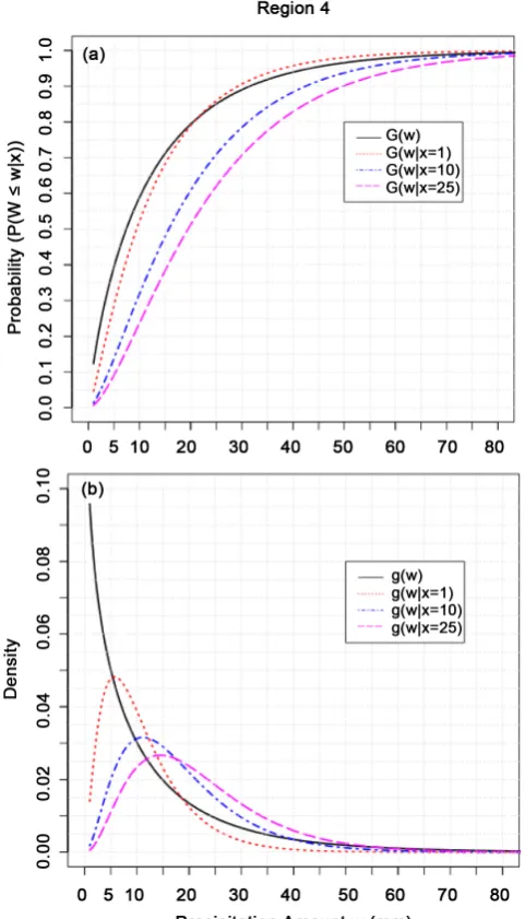
4.2.3. Region 4

[image:17.595.252.493.203.624.2]

(18)

posterior distributions functions. For simulated rainfall amount of 1 mm, the probability of observing less than or equal to 20 mm rainfall is 0.8; that is 80% chance.

The probability of observing rainfall amount greater than 20 mm is 0.2; 20% chance.

For simulated rainfall amount of 10 mm, the probability of observing rain-fall ≤ 20 mm is 0.6; that is 60% chance. The probability to observe rainrain-fall amount greater than 20 mm is 0.4. The probability of observing rainfall amounts ≤ 20 mm knowing that the simulated rainfall amount is 25 mm is 0.5 and the probability to observe rainfall greater than 20 mm is 0.5. Figure 11(b) shows that the most likely values of rainfall knowing that the simulated quantities for 1 mm, 5 mm and 25 mm are respectively 5 mm, 12 mm and 15 mm.

4.2.4. Region 5

posterior distributions functions. The probability of observing rainfall ≤ 10 mm for example knowing that the simulated quantity is 1 mm is 0.85; 85% chance. When the simulated quantities are 10 mm and 25 mm, the probability of serving rainfall ≤ 10 mm are 0.75and 0.72 respectively. The probability of ob-serving rainfall amounts greater than 10 mm are 0.25 and 0.28 respectively.

Fig-ure 12(b) shows that the most likely values which can be observed are between 3

and 5 mm for simulated rainfall amounts greater than 1 mm. It is noted that the most likely precipitations have low intensities. That means that heavy rainfalls are not recorded in the ocean during the JJAS season.

4.2.5. Region 6

For simulated rainfall amount of 1 mm, the probability of observing rainfall ≤ 20 mm is 0.8 and that to observe rainfall greater than 20 mm is 0.2 (see Figure

13(a)). When the simulated rainfall amounts are 10 mm and 25 mm, the

proba-bility of observing rainfall ≤ 20 mm are respectively 0.7 and 0.65 and those to observe rainfall greater than 20 mm are respectively 0.3 and 0.35. The most likely values of rainfall are 6 mm, 9 mm and 12 mm for simulated rainfall amounts of 1 mm, 10 mm and 25 mm respectively (see Figure 13(b)).

5. Conclusion

(19)

Figure 12. Examples of probabilistic forecasts of the precipitation amount W, conditional on precipitation occurrence, W greater than 0, and based on three different realizations x = 1, 10, 25 [mm] of predictor X for 24-h total precipitation amount output from the WRF model: (a) the prior (climatic) distribution function G and three posterior distribu-tion funcdistribu-tions G(w|x = 1), G(w|x = 10), G(w|x = 25); (b) the prior (cli-matic) density function g and three posterior density functions g(w|x = 1), g(w|x = 10), g(w|x = 25).

[image:19.595.237.509.74.565.2]

(20)

Figure 13. Examples of probabilistic forecasts of the precipitation amount W, conditional on precipitation occurrence, W greater than 0, and based on three diferent realizations x = 1, 10, 25 [mm] of predictor X for 24-h total precipitation amount output from the WRF model: (a) the prior (climatic) distribution function G and three posterior distribution functions G(w|x = 1), G(w|x = 10), G(w|x = 25); (b) the prior (climatic) density function g and three posterior density functions g(w|x = 1), g(w|x = 10), g(w|x = 25).

[image:20.595.238.509.80.553.2]

(21)

increases with simulated rainfall amounts. The forecasting functions determined in the present paper can be used by forecasters as guidance for issuing probabil-istic forecasts from a single determinprobabil-istic forecast. In addition, this forecasting tool might assist forecasters throughout the season in a wide variety of weather events.

Acknowledgements

WRF simulations were done on a workstation provided by Dr Serge Janicot of LOCEAN (Paris), in the framework of the PICREVAT project, funded by the French government. WRF was provided by the University Corporation for At-mospheric Research website (for more information see

http://www2.mmm.ucar.edu/wrf/users/download/get_source.html). GPCP data

were obtained from the NOAA website http://www.esrl.noaa.gov. TRMM data were provided online by NASA at http://mirador.gsfc.nasa.gov.

References

[1] Janicot, S. (1992) Spatiotemporal Variability of West African Rainfall. Part II: Asso-ciated Surface and Airmass Characteristics. Journal of Climate, 5, 499-511.

https://doi.org/10.1175/1520-0442(1992)005<0499:SVOWAR>2.0.CO;2

[2] Mkankam, K.F., Tsalefac, M. and Mbane, B.C. (1994) Variabilitépluviometrique sur le Territoire Camerounais: Essai de Régionalisation à Partir des Cumuls Mensuels et du Cycle Annuel. Publications de l'Association Internationale de Climatologie, 7, 439-446.

[3] Tchotchou, L.A.D. and Kamga, F.M. (2009) Sensitivity of the Simulated African Monsoon of Summers 1993 and 1999 to Convective Parameterization Schemes in RegCM3. Theoretical and Applied Climatology, 100, 207-220.

https://doi.org/10.1007/s00704-009-0181-2

[4] Tanessong, R.S., Vondou, D.A., Igri, P.M.F. and Mkankam, K. (2012) Evaluation of Eta Weather Forecast Model over Central Africa. Atmospheric & Climate Sciences, 2, 532-537. https://doi.org/10.4236/acs.2012.24048

[5] Trapero, L., Bech, J. and Lorente, J. (2012) Numerical Modelling of Heavy Precipi-tation Events over Eastern Pyrenees: Analysis of Orographic Effects. Atmospheric Research, 93, 408-418. https://doi.org/10.1016/j.atmosres.2009.01.021

[6] Richard, E., Buzzi, A. and Zangl, G. (2007) Quantitative Precipitation Forecasting in the Alps: The Advances Achieved by the Mesoscale Alpine Programme. Quarterly Journal of the Royal Meteorological Society, 133, 831-846.

https://doi.org/10.1002/qj.65

[7] Stensrud, D.J. and Yussouf, N. (2007) Reliable Probabilistic Quantitative Precipita-tion Forecasts Froma Short-Range Ensemble Forecasting System. Weather and Fo-recasting, 22, 2-17. https://doi.org/10.1175/WAF968.1

[8] Ullah, K. (2012) A Diagnostic Study of Convective Environment Leading to Heavy Rainfall during the Summer Monsoon 2010 over Pakistan. Atmospheric Research, 120, 226-239.

[9] Hamill, T.M. and Colucci, S.J. (1997) Veriﬁcation of Eta–Rsm Short-Range Ensem-ble Forecasts. Monthly Weather Review, 125, 1312-1327.

https://doi.org/10.1175/1520-0493(1997)125<1312:VOERSR>2.0.CO;2

(22)

Assessment: From Days to Decades. Quarterly Journal of the Royal Meteorological Society, 128, 747-774.https://doi.org/10.1256/0035900021643593

[11] Gneiting, T. and Raftery, A.E. (2005) Weather Forecasting Using Ensemble Me-thods. Science, 310, 248-249. https://doi.org/10.1126/science.1115255

[12] Glahn, H.R. and Lowry, D.A. (1972) The Use of Model Output Statistics (MOS) in Objective Weather Forecasting. Meteorology, 11, 1203-1211.

https://doi.org/10.1175/1520-0450(1972)011<1203:tuomos>2.0.co;2

[13] Bermowitz, R.J. (1975) An Application of Model Output Statistics to Forecasting Quantitative Precipitation. Monthly Weather Review, 103, 149-153.

https://doi.org/10.1175/1520-0493(1975)103<0149:AAOMOS>2.0.CO;2

[14] Antolik, M.S. (2000) An Overview of the National Weather Service’s Centralized Statistical Quantitative Precipitation Forecasts. Journal of Hydrology, 239, 306-337.

https://doi.org/10.1016/S0022-1694(00)00361-9

[15] Bremnes, J.B. (2004) Probabilistic Forecasts of Precipitation in Terms of Quantiles Using NWP Model Output. Monthly Weather Review, 132, 338-347.

https://doi.org/10.1175/1520-0493(2004)132<0338:PFOPIT>2.0.CO;2

[16] Friederichs, P. and Hense, A. (2007) Statistical Downscaling of Extreme Precipita-tion Events Using Censored Quantile Regression. Monthly Weather Review, 135, 2365-2378. https://doi.org/10.1175/MWR3403.1

[17] Applequist, S., Gahrs, G.E., Pfeﬀer, R.L. and Niu, X.F. (2002) Comparison of Me-thodologies for Probabilistic Quantitative Precipitation Forecasting. Weather and Forecasting, 17, 783-799.

https://doi.org/10.1175/1520-0434(2002)017<0783:COMFPQ>2.0.CO;2

[18] Hamill, T.M., Whitaker, J.S. and Wei, X. (2004) Ensemble Reforecasting: Improving Medium-Range Forecast Skill Using Retrospective Forecasts. Monthly Weather Re-view, 132, 1434-1447.

https://doi.org/10.1175/1520-0493(2004)132<1434:ERIMFS>2.0.CO;2

[19] Koizumi, K. (1999) An Objective Method to Modify Numerical Model Forecasts with Newly Given Weather Data Using an Artiﬁcial Neural Network. Weather and Forecasting, 14, 109-118.

https://doi.org/10.1175/1520-0434(1999)014<0109:AOMTMN>2.0.CO;2

[20] Ramirez, M.C., Velho, H.F.C. and Ferreira, N.J. (2005) Artiﬁcial Neural Network Technique for Rainfall Forecasting Applied to the Sao Paulo Region. Journal of Hy-drology, 301, 146-162. https://doi.org/10.1016/j.jhydrol.2004.06.028

[21] Gahrs, G.E., Applequist, S., Pfeﬀer, R.L. and Niu, X.F. (2003) Improved Results for Probabilistic Quantitative Precipitation Forecasting. Weather and Forecasting, 18, 879-890. https://doi.org/10.1175/1520-0434(2003)018<0879:IRFPQP>2.0.CO;2

[22] Yussouf, N. and Stensrud, D.J. (2006) Prediction of Near-Surface Variables at Inde-pendent Locations from a Bias-Corrected Ensemble Forecasting System. Monthly Weather Review, 134, 3415-3424. https://doi.org/10.1175/MWR3258.1

[23] Krzysztofowicz, R. and Maranzano, C.J. (2006) Bayesian Processor of Output for Probabilistic Quantitative Precipitation Forecasts. Systems Engineering and De-partment of Statistics, University of Virginia, Charlottesville.

[24] Wilks, D.S. (1990) Maximum Likelihood Estimation for the Gamma Distribution Using Data Containing Zeros. Journal of Climate, 3, 1495-1501.

https://doi.org/10.1175/1520-0442(1990)003<1495:MLEFTG>2.0.CO;2

[25] Hamill, T.M. and Colucci, S.J. (1998) Evaluation of Eta-RSM Ensemble Probabilistic Precipitation Forecasts. Monthly Weather Review, 126, 711-724.

(23)

[26] Wilson, L.J., Burrows, W.R. and Lanzinger, A. (1999) A Strategy for Verifying Weather Element Forecasts from an Ensemble Prediction System. Monthly Weather Review, 127, 956-970.

https://doi.org/10.1175/1520-0493(1999)127<0956:ASFVOW>2.0.CO;2

[27] Sloughter, J.M., Raftery, A.E., Gneiting, T. and Fraley, C. (2007) Probabilistic Quan-titative Precipitation Forecasting Using Bayesian Model Averaging. Monthly Weather Review, 135, 3209-3220. https://doi.org/10.1175/MWR3441.1

[28] Krzysztofowicz, R. (1983) Why Should a Forecaster and a Decision Maker Use Bayes Theorem. Water Resources Research, 19, 327-336.

https://doi.org/10.1029/WR019i002p00327

[29] Skamarock, W.C., Klemp, J.B., Dudhia, J., Gill, D.O., Barker, D.M., Wang, W. and Powers, J.G. (2008) A Description of the Advanced Research WRF Version 3. Na-tional Center for Atmospheric Research, Denver.

[30] Hong, S.Y., Pan, H.L. and Lim, J.O.J. (2006) The WRF Single—Moment 6-Class Microphysics Scheme (WSM 6). Asia-Pacific Journal of Atmospheric Sciences, 42, 129-151.

[31] Mlawer, E.J., Taubman, S.J., Brown, P.D., Iacono, M.J. and Clough, S.A. (1997) Ra-diative Transfer for Inhomogeneous Atmosphere: RRTM, a Validated Correlated-K Model for the Long-Wave. Journal of Geophysical Research, 102, 16663-16682.

https://doi.org/10.1029/97JD00237

[32] Tiedtke, M. (1989) A Comprehensive Mass Flux Scheme for Cumulus Parameteri-zation in Large Scale Models. Mon. Monthly Weather Review, 117, 1779-

1800. https://doi.org/10.1175/1520-0493(1989)117<1779:ACMFSF>2.0.CO;2

[33] Nordeng, T.E. (1994) Extended Versions of the Convective Parameterization Scheme at ECMWF and Their Impact on the Mean and Transient Activity of the Model in the Tropics. ECMWF Technical Memorandum, 206, 41.

[34] Huﬀman, G.J., Morrissey, M., Bolvin, D., Curtis, S., Joyce, R., McGavock, B., Suss-kind, J. and Adler, R.F. (2001) Global Precipitation at One Degree Daily Resolution from Multisatellite Observations. Journal of Hydrometeorology, 2, 36-

50. https://doi.org/10.1175/1525-7541(2001)002<0036:GPAODD>2.0.CO;2

[35] Gong, X. and Richman, M.B. (1995) On the Application of Cluster Analysis to Growing Season Precipitation Data in North America East of the Rockies. Journal of Climate, 8, 897-931.

https://doi.org/10.1175/1520-0442(1995)008<0897:OTAOCA>2.0.CO;2

[36] Unal, Y., Kindap, T. and Karaca, M. (2003) Redeﬁning the Climate Zones of Turkey Using Cluster Analysis. International Journal of Climatology, 23, 1045-1055.

https://doi.org/10.1002/joc.910

[37] Rao, A.R. and Srinivas, V.V. (2006) Regionalization of Watersheds by Hybr-id-Cluster Analysis. Journal of Hydrology, 318, 37-56.

https://doi.org/10.1016/j.jhydrol.2005.06.004

[38] Yepdo, D.Z., Monkam, D. and Lenouo, A. (2009) Spatial Variability of Rainfall Re-gions in West Africa during the 20th Century. Atmospheric Science Letters, 10, 9-13. https://doi.org/10.1002/asl.202

[39] Dezfuli, A.K. (2011) Spatio-Temporal Variability of Seasonal Rainfall in Western Equatorial Africa. Theoretical and Applied Climatology, 104, 57-69.

https://doi.org/10.1007/s00704-010-0321-8

(24)

Estimates with a High-Density Gauge Dataset for West Africa. Part II: Validation of TRMM Rainfall Products. Journal of Applied Meteorology, 42, 1355-1368.

https://doi.org/10.1175/1520-0450(2003)042<1355:VOTAOR>2.0.CO;2

[41] Huﬀman, G., Adler, R., Arkin, P., Chang, A., Ferraro, R., Gruber, A., Janowiak, J., Mc-Nab, A., Rudolf, B. and Schneider, U. (1997) The Global Precipitation Clima-tology Project (GPCP) Combined Precipitation Dataset. Bulletin of the American Meteorological Society, 78, 5-20.

https://doi.org/10.1175/1520-0477(1997)078<0005:TGPCPG>2.0.CO;2

[42] Arkin, P.A. and Meisner, B.N. (1987) The Relationship between Large Scale Con-vective Rainfall and Cold Cloud over the Western Hemisphere during 1982-84. Monthly Weather Review, 115, 51-74.

https://doi.org/10.1175/1520-0493(1987)115<0051:TRBLSC>2.0.CO;2

[43] Kelly, K.S. and Krzysztofowicz, R. (1995) A Bivariate Meta-Gaussian Density for Use in Hydrology. Stochastic Hydrology and Hydraulics, 11, 17-31.

https://doi.org/10.1007/BF02428423

[44] Krzysztofowicz, R. and Herr, H.D. (2001) Hydrologic Uncertainty Processor for Probabilistic River Stage Forecasting: Precipitation-Dependent Model. Journal of Hydrology, 249, 46-68. https://doi.org/10.1016/S0022-1694(01)00412-7

[45] Krzysztofowicz, R. (2002) Bayesian System for Probabilistic River Stage Forecasting. Journal of Hydrology, 268, 16-40. https://doi.org/10.1016/S0022-1694(02)00106-3

[46] Tanessong, R.S., Vondou, D.A., Moudi-Igri, P., Kamsu-Tamo, P.H. and Mkan-kam-Kamga, F. (2013) Evaluation of Probabilistic Precipitation Forecast Deter-mined from WRF Forecasted Amounts. Theoretical and Applied Climatology, 116, 649-659. https://doi.org/10.1007/s00704-013-0965-2

Submit or recommend next manuscript to SCIRP and we will provide best service for you:

Accepting pre-submission inquiries through Email, Facebook, LinkedIn, Twitter, etc. A wide selection of journals (inclusive of 9 subjects, more than 200 journals)

Providing 24-hour high-quality service User-friendly online submission system Fair and swift peer-review system

Efficient typesetting and proofreading procedure

Display of the result of downloads and visits, as well as the number of cited articles Maximum dissemination of your research work