An Innovative Genetic Algorithms Based Inexact Non Linear Programming Problem Solving Method

http://www.scirp.org/journal/jep ISSN Online: 2152-2219

ISSN Print: 2152-2197

An Innovative Genetic Algorithms-Based

Inexact Non-Linear Programming Problem

Solving Method

Weihua Jin, Zhiying Hu, Christine Chan

Energy Informatics Laboratory, Faculty of Engineering & Applied Science. University of Regina, Regina, SK, Canada

Abstract

In this paper, an innovative Genetic Algorithms (GA)-based inexact non-linear programming (GAINLP) problem solving approach has been proposed for solving non-linear programming optimization problems with inexact informa-tion (inexact non-linear operainforma-tion programming). GAINLP was developed based on a GA-based inexact quadratic solving method. The Genetic Algo-rithm Solver of the Global Optimization Toolbox (GASGOT) developed by MATLABTM _{was adopted as the implementation environment of this study.}

GAINLP was applied to a municipality solid waste management case. The re-sults from different scenarios indicated that the proposed GA-based heuristic optimization approach was able to generate a solution for a complicated non-linear problem, which also involved uncertainty.

Keywords

Genetic Algorithms, Inexact Non-Linear Programming (INLP), Economy of Scale, Numeric Optimization, Solid Waste Management

1. Introduction

Municipal solid waste management involves activities such as waste collection, transportation, treatment, reutilization, and disposal. Economic optimization in the operation programming of solid waste management was first proposed in the 1960s [1]. Different models of waste planning have been researched and applied in various engineering fields in the following decades. The primary considerations involved are cost control, environmental sustainability and waste reutilization. The techniques employed include linear programming [2][3][4][5], mixed integer linear programming [6], multi-objective programming [7][8][9], nonlinear pro-gramming [10][11], as well as their hybrids, which involve probability, fuzzy set

How to cite this paper: Jin, W.H., Hu, Z.Y. and Chan, C. (2017) An Innovative Genetic Algorithms-Based Inexact Non-Li- near Programming Problem Solving Me-thod. Journal of Environmental Protection, 8, 231-249.

https://doi.org/10.4236/jep.2017.83018

Received: October 13, 2016 Accepted: March 11, 2017 Published: March 14, 2017

Copyright © 2017 by authors and Scientific Research Publishing Inc. This work is licensed under the Creative Commons Attribution International License (CC BY 4.0).

and inexact analysis [12][13][14][15][16]. Due to complexity of the problem, research reports on nonlinear programming problems for solid waste management are scarce; some exceptions are [17][18]. In some of the works such as [10][11], the nonlinear objective functions are converted into linear functions or simplified into quadratic functions under some adopted conditions and assumptions.

The approach of operational programming with inexact analysis often treats the uncertain parameters as intervals with known lower and upper bounds and un-clear distributions. A major advantage of inexact programming is that the varia-tion in system performance and decision variables can be investigated by solving relatively simple sub-models. In real-life problems, while the available information is often inadequate and the distribution functions are often unknown, it is gener-ally possible to represent the obtained data with inexact numbers that can be rea-dily used in the inexact programming models. For decision makers, it is usually more feasible to represent uncertain information as inexact data than to specify distributions of fuzzy sets or probability functions. Hence, various kinds of inexact programmings such as inexact linear programming (ILP), inexact quadratic pro-gramming (IQP), inexact integer propro-gramming (IIP), inexact dynamic program-ming (IDP) and inexact multi-objective programprogram-ming (IMOP) have been devel-oped and are well discussed [10][11][19][20][21][22]. It can be observed from these studies that applications of inexact models to practical solid waste planning systems are effective.

In [23], the approach of GA for ILP and IQP is discussed; the comparisons of traditional binary analysis solving methods [8] [21] [22] [24] with GA-based methods indicate that for ILP and IQP, GA can generate better results with less computational complexity.

In the literature, much work on traditional binary analysis for IQP has been done, for example, see [10][11] [21] [22]. However, traditional binary analysis methods for ILP and IQP involve unavoidable simplifications and assumptions, which often increased the chance for error in the problem solving process and adversely affected the quality of the results. Moreover, a more complex model often increases error in the solution. However, it has been observed that more complex models often produce less optimal results, and studies that focus on in-exact nonlinear programming problems are scarce. For example, in [19], the me- thodology is mainly focused on combining endpoint values of the inexact para-meters to form a set of deterministic problems, which will only work for partic-ular monotone functions within a small scale model. Therefore, a more flexible problem solving method for the general INLP is desired.

This paper is organized as follows. Section 2 presents the background of the research, which includes an introduction to the problem of Solid Waste Man-agement (SWM), the concept of economies of scale in SWM, and the concept of GA, and the Genetic Algorithm Non-Linear Solver Engine (GANLP) that is used for implementing the proposed method. Section 3 discusses the methodology of the proposed GA-based methods for solving inexact non-liner problems. Section 4 presents a case study in which the solutions for different scenarios of the INLP problem of solid waste disposal planning are generated.

2. Background

2.1. Solid Waste Management and the Concept of Economy of

Scale in Solid Waste Management Planning

Solid waste management is the process of removing waste materials from the su- rrounding environment, which involves the collection, separation, storage, pro- cessing, treatment, transport, recovery and disposal of solid waste. Landfill and incineration are two of the most commonly used solid waste disposal methods. The objective of a solid waste management process is to dispose of discarded materials in a timely manner so as to prevent the spread of disease, minimize the likelihood of contamination, and reduce their effects on human health and the environment.

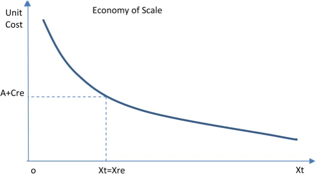
The economy of scale (ES) is a microeconomics term, and it refers to the ad-vantages that enterprises obtain due to their size or scale of operation, with the cost per unit of output generally decreasing as the scale increases and fixed costs are distributed over more units of output. In a solid waste management system, ES exists within the transportation process [25] and it can be expressed as a siz-ing model with a power law [11].

(

)

t re t re

C =C X X + (1)

where X_t

( )

( )

waste flow; C_t

( )

( )

t

X ; C_re

( )

scale to the unit cost of waste transportation for reference waste flow X_re

( )

0

re

C < ; and m is an economy of scale exponent which reflects the unit cost

de-cline with respect to the waste flow, − <1 m<0.

Thus the cost function for waste transportation can be expressed as,

(

)

t t

C=X A+C (2)

where C

( )

( )

fixed unit charge, and A C+ t is the unit transportation cost. The unit

trans-portation cost affected by ES is shown in Figure 1.

Figure 1. Unit transportation cost affected by ES.

In the next section, the concept of GA is introduced.

2.2. GA for Solving Non-Linear Problems (GANLP)

2.2.1. GA for Deterministic Optimization Problems

A generic procedure of GA can be summarized as follows:

1) Initialization: The initialization step involves establishing the mapping mode between the genotype and phenotype; this can be done by determining the cod-ing and decodcod-ing functions, creatcod-ing the fitness function accordcod-ing to the objec-tive of the problem domain, and generating the initial population Pop0 with a

size of N. In GA, the term genotype refers to a candidate solution for a

prob-lem, which is often encoded as a bit string, while the phenotype is a domain so-lution itself and is encoded to be a genotype [26]. This process can be carried out randomly or can be guided by domain information.

2) Evaluation: This step involves calculating the fitness value of each individu-al in the population Popt.

3) Selection: This step involves applying a selection operator to the population

t

Pop .

4) Elitism: This step involves selecting and preserving the elitist individual in the population.

5) Crossover: This step involves applying a crossover operator to the popula-tion Popt.

6) Mutation: This step involves applying a mutation operator to the population

t

Pop and creating the next generation’s population Popt+1.

7) Termination test: This step involves checking whether a satisfactory solu-tion has been found, or the preset terminasolu-tion condisolu-tion is met; if one of the con-dition is true, the algorithm is terminated. Otherwise, the procedure loops back to step (2).

This generic procedure of GA is illustrated as a flowchart in Figure 2.

Figure 2. Flowchart of procedure of GA.

efficient for engineering applications. Among these implementations, the Ge-netic Algorithm Solver of the Global Optimization Toolbox (GASGOT) imple-ments a simulated evolution in the MatlabTM _{(Trademark of MathWord)}

envi-ronment by using both binary and floating-point representations. GASGOT was developed by the Department of Industrial Engineering of North Carolina State University. This implementation provides a flexible platform of genetic operators, selection functions, termination functions, and the evaluation [27]. GASGOT runs in the MatlabTM _{workspace and can be easily invoked by other programs.}

GASGOT supports both binary and floating-point representations, and the cor-responding genetic operators have been developed. This study adopts GASGOT as the implementation tool of GA, and the applications and numeric examples were calculated in MatlabTM _{based on the GA non-linear program (GANLP) solver}

engine of GASGOT.

2.2.2. GA for Problem Solving of Non-Linear Problems (GANLP)

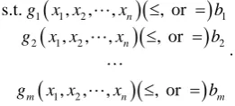
A general non-linear programming problem (NLP) can be expressed as follows

[28]:

(

)

(

)(

)

(

)(

)

(

)(

)

1 1 2 1

2 1 2 2

1 2

s.t. , , , , or

, , , , or

.

, , , , or

n

n

m n m

g x x x b

g x x x b

g x x x b

≤ =

≤ =

≤ =

 

 

[28] indicated that some specially formed non-linear programming problems can be solved by calculus-based algorithms, which assume that the objective function f x

( )

differen-tiable functions of x. Most calculus-based methods aim to transform the non-

linear problem into a sequence of solvable sub-problems. The methods generally require explicit or implicit second derivative calculations of the objective func-tion, which in some of the methods can be ill-conditioned and can cause the al-gorithm to fail [29]. This weakness in the calculus-based method has prompted many researchers to propose GA, which is a random search method, for solving non-linear programming problems [30][31].

The following example is taken from [28]:

(

)

(

)

1 1 2 2 1 2

Max 30z=x −x +x 35−x −x −2x (4)

2 2

1 2

1 2

1 2

s.t. 2 250

20

, 0.

x x x x x x

+ ≤

+ ≤

≥

This problem, similar to many NLPs, can be formulated as follows:

( )

1

Max z=

∑

( )

(

)

s.t. 1, 2, , .

n

ij j i j i

g x b i m

=

≤ =

∑

Since the decision variables appear separate in terms of the objective function and the constraints, NLPs of this form are called separable programming problems. This kind of NLP can be solved by approximating each fj

( )

( )

using a piecewise linear function [28].

The approximating problem for the above example Equation (4) gives the re-sult x1=5, 5, 200x2= z= , while the actual optimal solution is

1 7.5, 5.83, 214.58.2

x = x = z=

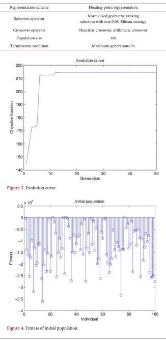
A GA program for the above example has been constructed with the parame-ters specified in Table 1.

The result given by the GA program is: x1=7.499, x2 =5.8352, z=214.58.

The evolution curve is shown as Figure 3. Compared to the results generated using the calculus-based method of [28], the GA generated results are closer to the actual optimal solution.

In Figure 3, it can be seen that at approximately the 15th generation, the

optim-al solution was generated. Although the fitness of the initioptim-al population shown in

Figure 4 is not excellent, compared to the separable programming technique

Table 1. Parameters of genetic algorithms.

Representation scheme Floating-point representation

Selection operator _{selection with rate 0.08, Elitism strategy} Normalized geometric ranking

Crossover operator Heuristic crossover, arithmetic crossover

Population size 100

Termination condition Maximum generations 50

Figure 3. Evolution curve.

3. GA for Problem Solving of Inexact Non-Linear Problems

(GAINLP)

Quadratic programming problems are specific cases of non-linear programming problems [23]. Due to the lack of generally applicable algorithms for handling the non-linear structure, and the inexact information embedded in the structure, most non-linear programming problems are difficult to solve. The engine for solving interactive binary analysis based inexact linear problems proposed in [21][22] is not intended for dealing with generic non-linear problems. By contrast, GA can be used as a general problem solver for this type of problems because there is not much difference for GA between treating the term of 2

i

x in quadratic

program-ming problems and the terms x xi j or

0.28

i

x in generic non-linear

program-ming problems.

[23] has proposed a method for solving the IQP problem, which can be mod-ified to solve generic inexact non-linear programming problems. The GA-based inexact non-linear programming method GAINLP involves three stages of prob-lem solving. In the following, a computation experiment will be conducted to il-lustrate how the GAINLP method can handle complicated inexact non-linear problems Equation (6).

( )

(

)

1 1 2 1 1 2 2 1 2

Max f±=c x± ±−c± x± −d x± ±+d± x x± ± (6)

( )

11 1 12 2 1

1 2 2 2

s.t.

j 0, 1, 2

a x a x b

x a x b

x j ± ± ± ± ± ± ± ± ± ± + ≤ + ≤ ≥ =

where a b c dij, i, j, j

± ± ± ±

are inexact parameters and xj

±

is an inexact variable, for an inexact number g±∈ g−,g+_, g+ and g− are the upper and lower

bounds, respectively. In this experiment,

[

]

[

]

[ ]

1, 1 16,18 ; 2, 2 12,14 ; 1, 1 4, 5 ;

c c− + c c− + d− d+

 =  =  =

     

[

]

[

]

[

]

2, 2 14,15 ; 11, 11 4.5, 5.5 ; 12, 12 1.8, 2.2 ;

d− d+ a− a+ a− a+

 =  =  =

     

[

]

[

]

[

]

1, 1 1.8, 2.1 ; 2, 2 1.8, 2.2 ; 2, 2 0.9,1.1 .

b b− + a a− + b b− +

 =  =  =

     

GAINLP has been designed to include three stages of problem solving. In stage one, to obtain the initial suboptimal s

j

x , the random numbers of , , ,

r r r r ij i j j

a b c d were selected to transfer this INLP problem to a NLP problem, such

that a b c dijr, ir, rj, rj satisfy the continuous uniform distribution in the intervals of

, , , , ,

ij ij i i j j

a a− + b b− + c c− +

     

      and dj,dj

− +

 

 .

( )

( )

1 1 2 1 1 2 2 1 2

Max fs =c xr s−cr xs −d xr s+dr x xs s (7)

( )

11 1 12 2 1

1 2 2 2

s.t.

0, 1, 2.

r s r s r s r s r

s j

a x a x b

x a x b

x j

+ ≤

+ ≤

Then, the heuristic search algorithm of the GANLP solver engine, presented in Section 2.2, can be used to identify a suboptimal solution _fs, and the

cor-responding decision variable s j

x . The objective function in Equation (7) was

used as the positive term of the fitness function and the constraints of Equation (6) adopted as the negative punishment terms. The result is:

1 0.346, 0.171, 2.296.2

s s s

x = x = f = −

In stage two, by substituting 1, 2

s s

x x into Equation (6), the inexact coefficients

of a b c d_ij±, _i±, ±_j, _j± will be determined. There are two kinds of decision schemes for inexact programming problems, the conservative scheme and optimistic scheme [20]. The former assumes less risk than the latter, so that for a maximi-zation objective function, planning for the lower bound of an objective value

f− represents the conservative scheme, and planning for the upper bound of an

objective value f+ represents the optimistic scheme [20]. In terms of constraints,

the conservative scheme involves more rigorous or stringent constraints, and the optimistic scheme adopts more tolerant ones.

The 1, 2

s s

x x obtained in stage one are used to construct two optimization pro-

blems in order to determine the coefficients of aij ,bi ,cj ,dj

±+ ±+ ±+ ±+

and , , ,

ij i j j

a±− b±− c±− d±− respectively. The coefficients from the first group are

consi-dered to be corresponding to the optimistic scheme f+, while the second group

correspond to the conservative scheme f−. Considering c dj, j

± ±

are variables, the following two functions can be constructed:

( )

( )

1 1 2 1 1 2 2 1 2

Max s s s s s

f+ =c x±+ −c±+ x −d±+x +d±+ x x (8)

[

]

[

]

[ ]

[

]

( )

( )

1 1 2 1 1 2 2 1 2

Min f− =c x±− s−c±− xs −d±−xs+d±− x xs s (9)

[

]

[

]

[ ]

[

]

To determine aij ,bi

+ +

± ± _{of the optimistic scheme in correspondence with the}

upper limit of the objective value f+, the objective function can be constructed

as follows:

( )

(

)

11 1 12 2 1

Max s s

abs a± x +a x± −b± (10)

( )

11 1 12 2 1

s.t. a± xs +a x± s ≤b±

(

)

1 2 2 2

Max

s.t. ,

s s s s

abs x a x b

x a x b

± ±

± ±

+ −

+ ≤

The objective functions to get aij ,bi

− −

± ± _{of the conservative scheme are:}

( )

(

)

11 1 12 2 1

Min abs a± xs +a x± s−b± (11)

( )

11 1 12 2 1

s.t. s s

a± x +a x± ≤b±

and

(

)

1 2 2 2

Min

s.t. .

s s s s

abs x a x b

x a x b

± ±

± ±

+ −

+ ≤

By solving the above functions Equations (8)-(11), the values of all the inexact coefficients are obtained, such that,

11 4.5, 12 1.8, 1 2.1, 2 1.8, 2 1.1

a±+ = a±+ = b±− = a±+ = b±+ =

11 5.5, 12 2.2, 1 1.8, 2 2.2, 2 0.9

a±− = a±− = b±− = a±− = b±− =

1 18, 2 12, 1 4, 2 15

c±+ = c±+ = d±+ = d±+= ;

1 16, 2 14, 1 5, 2 14

c±−= c±− = d±−= d±−= .

In stage three, the objective function presented in Equation (7) is converted into the following two sub-problems:

( )

(

)

( )

0.3

1 1 2 1 2

0.5

1 2

1 2

1 2

Max 18 12 4 15 ,

s.t. 4.5 1.8 2.1,

1.8 1.1,

0, 0,

f x x x x x

x x x x x x + ± ± ± ± ± ± ± ± ± ± ± = − − + + ≤ + ≤ ≥ ≥ and

( )

(

)

( )

1 1 2 1 2

0.5

1 2

1 2

1 2

Max 16 14 5 14 ,

s.t. 5.5 2.2 1.8,

2.2 0.9,

0, 0.

f x x x x x

x x x x x x − ± ± ± ± ± ± ± ± ± ± ± = − − + + ≤ + ≤ ≥ ≥

In this stage, the inexact parameters in Equation (7) have been eliminated, and two typical non-linear optimization problems have been generated instead. Solving the above two objective functions by GANLP, the solution of the exam-ple Equation (6) is:

[

]

f±= − − , x1

[

]

± ₌

, and x2

[

]

± ₌

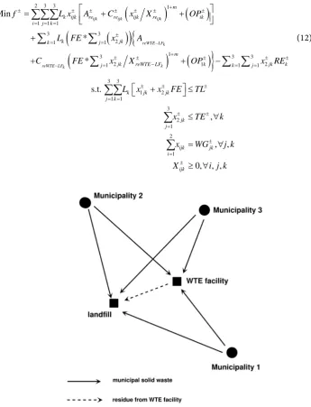
4. Case Study

The study region includes three municipalities, a waste-to-energy (WTE) facility and a landfill, as shown in Figure 5. Three time periods are considered; each has an interval of five years. Over the 15 year planning horizon, an existing landfill and WTE facilities are available to serve the municipal solid waste (MSW) disposal needs in the region. The landfill has an existing capacity of

[

]

2.05, 2.30 ×10 t, and the WTE facility has a capacity of

[

]

streams, and its revenue from energy sale is

[

]

Table 2 shows the waste generation rates of the three municipalities and the

operating costs of the two facilities in the three periods.

Taking into consideration the effects of the ES, the inexact non-linear (INLP) model can be formulated as follows:

(

)

( )

( )

(

){

(

)

( )

}

2 3 3 1

3 3

2

1 1

1

3 3 3

2 1 2

1 1 1

1 1 1

Min

*

*

ijk ijk ijk

reWTE LFk

reWTE LFk k

m

k ijk re re ijk re ik

k jk

k j

m

jk reWTE LF k jk k

j j

j k

k i

f L x A C x X OP

L FE x A

C FE x X OP x RE

− − + ± ± ± ± ± ± ± ± = = + ± ± ± ± ± − = = = = = =      =  + + + + + −

∑∑∑

∑

∑

∑

∑ ∑

k jk jk j k j i jk ijk jk ijk

L x x FE TL

x TE k

x WG j k

X i j k

± ± ± ± = = = ± ± = ±  + ≤   ≤ ∀ = ∀ ≥ ∀

∑∑

∑

∑

Table 2. Data for the waste generation and treatment/disposal.

Time Period

1

k= k=2 k=3

Waste generation WGjk( )t d

±

Municipality 1(j=1) [260, 340] [310, 390] [360, 440]

Municipality 2(j=2) [160, 240] [185, 265] [210, 290]

Municipality 3(j=3) [260, 340] [260, 340] [310, 390]

Operation cost OPik( )$ t

±

Landfill (i=1) [30, 45] [40, 60] [50, 80]

WTE Facility (i=2) [55, 75] [60, 85] [65, 95]

where, i is the type of waste management facility (i=1, 2, where i=1 for

land-fill, 2 for WTE); j is the city, j=1, 2, 3; k is the time period, k=1, 2, 3; Lk

is the length of period k, L1=L2=L3=365*5 (day); OP_ik± is the operating

cost of facility iduring period k

( )

period k ($/t), RE1 RE2 RE3

[

]

± ₌ ±₌ ± ₌

; TE± is the capacity of WTE

(t/d); TL± is the capacity of the landfill (t); WGjk

± _{is the waste disposal demand}

in city j during period k

( )

±

is the waste flow from city j to facility

i during period k

( )

In this objective function Equation (12), the first term on the right side reflects the transportation costs in each management period (k = 1 to 3) from each city to each waste treatment unit, and the related operation costs. The second term reflects the cost incurred in transporting the products from the WTE facility to the landfill, and the operation cost at the landfill. The third term is the revenue generated from the WTE facility.

The MSW generation rates generally vary between different municipalities and for different periods, and the costs for the waste transportation and treat-ment also vary temporally and spatially. Furthermore, interactions exist between the waste flows and their transportation costs due to the effects of the ES. Tables 3-5 show the parameters related to the economy of scale, which include the fixed unit transportation cost Are, the reference waste flow Xre and the coefficient

Crecorresponding to Xre.

Hence, it can be observed that the traditional methods of binary analysis can-not solve this problem without additional assumptions or simplifications. The following discussion will explain how traditional methods solve this problem by simplifying the non-linear effects of the ES.

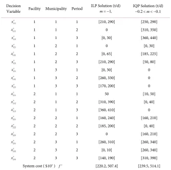
Scenario (i) Letting m= −1, the effects of the ES are totally ignored. This

converts the inexact non-linear programming (INLP) problem to an inexact li-near programming (ILP) problem, and the GAILP method presented in [23] can solve the problem.

Scenario (ii) Assuming −0.2<m< −0.1, it is indicated that the non-linear

Table 3. Fixed unit transportation costs.

City-to-landfill fixed unit transportation cost Are1jk( )$ t

±

11k

re

A± _{[14.58, 19.40] [16.04, 21.34] [17.64, 23.48]}

12k

re

A± [12.65, 16.87] [13.92, 18.56] [15.31, 20.41]

13k

re

A± [15.30, 20.49] [16.83, 22.53] [18.52, 24.79]

City-to-WTE fixed unit transportation cost Are2jk( )$ t

±

21k

re

A± [11.57, 15.42] [12.73, 16.97] [14.00, 18.66]

22k

re

A± [12.17, 16.15] [13.39, 17.76] [14.73, 19.54]

23k

re

A± _{[10.60, 14.10] [11.67, 15.51] [12.83, 17.06]}

WTE-to-landfill fixed unit transportation cost ( )$ t reWTE LFk A

−

±

[5.71, 7.62] [6.28, 8.38] [6.91, 9.33]

Table 4. Reference waste flow.

City-to-landfill reference waste flow Xre1jk( )t d

±

11k

re

X± [220, 250] [240, 280] [260, 320]

12k

re

X± _{[160, 200] [180, 220] [220, 260]}

13k

re

X± [160, 200] [180, 240] [200, 240]

City-to-WTEreference waste flow Xre2jk( )t d

±

21k

re

X± _{[200, 240] [240, 280] [280, 320]}

22k

re

X± [120, 170] [150, 190] [180, 220]

23k

re

X± [220, 270] [220, 270] [240, 270]

WTE-to-landfill reference waste flow ( )t d k

reWTE LF

X± −

[170, 200] [200, 260] [240, 270]

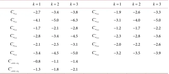
Table 5. C_re

( )

1

k= k=2 k=3 k=1 k=2 k=3

11k

re

C− −2.7 −3.4 −3.8

21k

re

C− −1.9 −2.6 −3.3

11k

re

C+ _{−4.1 −5.0 −6.3}

21k

re

C+ _{−3.1 −4.0 −5.0}

12k

re

C− −1.7 −2.1 −2.8 Cre22k

−

−1.2 −1.7 −2.2

12k

re

C+ _{−2.8 −3.4 −4.5}

22k

re

C+ _{−2.3 −2.8 −3.6}

13 k

re

C− −2.1 −2.5 −3.1 Cre23k

−

−2.0 −2.2 −2.6

13k

re

C+ −3.4 −4.5 −5.0

23k

re

C+ −3.2 −3.5 −3.9

reWTE LFk

C− ₋ −0.8 −1.1 −1.4

reWTE LFk

C+ ₋ −1.3 −1.8 −2.1

Note: The + and –superscript sign of Cre represents the value of Cre relevant to the upper and lower bound of Xre only.

problem is converted into an inexact quadratic programming problem.

Table 6 lists the solutions of the objective function Equation (12) for above

two scenarios (i) and (ii).

the value of m deviates away from the predetermined value, this inaccuracy will increase dramatically.

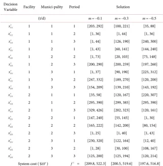
Applying the GAINLP model on the inexact non-linear programming prob-lem, the optimization problem represented in Equation (12) can be solved di-rectly without additional assumptions for the effects of the ES. By adopting this approach, the solution can be found even when the ES exponent m is not within the interval of

[

]

Three different scenarios, m= −0.1, 0.3, 0.5m= − m= − have been tested,

and the solutions given by the GAINLP model are shown in Table 7.

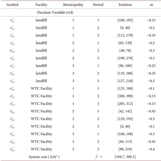
The above scenarios assume that the economy of scale exponent is universal in the whole region during the entire period. However, this is not always necessari-ly true for practical engineering problems. More common situations may involve different scale exponents for various combinations of municipalities and facilities in different periods. Thus, Table 8 illustrates the solutions for the fourth scenario, which involves different scale exponents.

In the objective function of the inexact non-linear programming model Equa-tion (12), the weight of the transportaEqua-tion cost in the system operaEqua-tion cost va-ries according to different Ct values. The effect becomes significant when waste

Table 6. Solutions obtained by applying the ILP model (m= −1) and IQP model (−0.2<m< −0.1).

Decision

Variable Facility Municipality Period ILP Solution (t/d) m= −1,

IQP Solution (t/d)

0.2 m 0.1

− < < −

111

x± 1 1 1 [210, 290] [250, 290]

112

x± 1 1 2 0 [310, 350]

113

x± 1 1 3 [0, 30] [360, 440]

121

x± 1 2 1 0 [0, 30]

122

x± 1 2 2 [0, 65] [185, 225]

123

x± 1 2 3 [210, 290] [50, 80]

131

x± 1 3 1 [0, 30] 0

132

x± 1 3 2 [260, 330] 0

133

x± 1 3 3 [170, 200] 0

211

x± 2 1 1 50 [10, 50]

212

x± 2 1 2 [310, 390] [0, 40]

213

x± 2 1 3 [360, 410] 0

221

x± 2 2 1 [160, 240] [160, 210]

222

x± 2 2 2 [185, 200] [0, 40]

223

x± 2 2 3 0 [160, 210]

231

x± 2 3 1 [260, 310] [260, 340]

232

x± 2 3 2 [0, 10] [260, 340]

233

x± 2 3 3 [140, 190] [310, 390]

System cost ( 6

$10 ) f± [220.2, 507.4] [239.5, 514.1]

Table 7. Solutions when m= −0.1, 0.3 and 0.5.

Decision

Variable Facility Munici-pality Period Solution

(t/d) m= −0.1 m= −0.3 m= −0.5

111

x± 1 1 1 [203, 292] [100, 221] [35, 88]

112

x± 1 1 2 [1, 36] [1, 44] [1, 36]

113

x± 1 1 3 [1, 44] [126, 190] [240, 300]

121

x± 1 2 1 [1, 43] [60, 141] [144, 240]

122

x± 1 2 2 [1, 73] [20, 103] [75, 148]

123

x± 1 2 3 [200, 290] [200, 259] [197, 260]

131

x± 1 3 1 [1, 37] [90, 190] [225, 312]

132

x± 1 3 2 [247, 332] [189, 270] [120, 200]

133

x± 1 3 3 [154, 209] [139, 210] [143, 192]

211

x± 2 1 1 [35, 58] [120, 167] [220, 307]

212

x± 2 1 2 [295, 390] [299, 385] [295, 390]

213

x± 2 1 3 [329, 426] [202, 323] [120, 161]

221

x± 2 2 1 [147, 240] [55, 145] [1, 30]

222

x± 2 2 2 [165, 222] [142, 200] [80, 154]

223

x± 2 2 3 [1, 25] [1, 40] [1, 43]

231

x± 2 3 1 [230, 320] [122, 164] [12, 40]

232

x± 2 3 2 [1, 28] [30, 100] [108, 167]

233

x± 2 3 3 [125, 200] [125, 194] [120, 214]

System cost ( 6

$10 ) f± _{= [209.8, 522.3] [200.5, 519.6] [197.6, 516.8]}

Note: Facility: 1 = landfill, 2 = WTC Facility.

flow becomes lower and the hauling distances are substantial. This effect is a non- linear function of the waste flow xijk, in which the reference waste flow xre and

the economy of scale exponent m are the parameters. Thus, the problem is a complicated non-linear programming problem, and the GA-based search ap-proach has been shown to be adequate for solving this kind of economy optimi-zation problems.

It is also reasonable to assume that between different locations

(i=1, 2; 1, 2, 3j= ), for different time periods (k=1, 2, 3), the economy of scale exponent (mijk and mWTE−LFk) may be different, since m is the parameter

used to describe the characteristics and attributes of a particular transportation scenario. Under these considerations, scenario 4 was designed with different op-eration costs and transportation strategies. On the other hand, the traditional inexact linear and inexact quadratic programming methods will not be able to handle situations like scenario 4 without additional assumptions and simplifica-tion.

The results also show that when the value of the economy of scale exponentm

becomes smaller, from −0.1, −0.3 to −0.5, for both f positive scheme and f

Table 8. Solutions when m is different for each municipality and each period.

Symbol Facility Municipality Period Solution m

Decision Variable (t/d)

111

x± landfill 1 1 [100, 192] −0.15

112

x± landfill 1 2 [0, 40] −0.2

113

x± landfill 1 3 [112, 178] −0.35

121

x± landfill 2 1 [65, 139] −0.2

122

x± landfill 2 2 [40, 78] −0.3

123

x± landfill 2 3 [199, 279] −0.3

131

x± landfill 3 1 [90, 189] −0.25

132

x± landfill 3 2 [135, 280] −0.25

133

x± landfill 3 3 [127, 218] −0.3

211

x± WTC Facility 1 1 [125, 189] −0.1

212

x± WTC Facility 1 2 [300, 390] −0.15

213

x± WTC Facility 1 3 [205, 312] −0.15

221

x± WTC Facility 2 1 [42, 142] −0.45

222

x± WTC Facility 2 2 [129, 192] −0.3

223

x± WTC Facility 2 3 [0, 40] −0.1

231

x± WTC Facility 3 1 [100, 198] −0.3

232

x± WTC Facility 3 2 [44, 113] −0.45

233

x± WTC Facility 3 3 [99, 219] −0.4

System cost ( 6

$10 ) f±= [194.7, 500.1]

Note: for transportation from WTE facility to landfill, m = −0.5.

smaller. At the same time, the range of the intervals of the minimized objective function also decreases. This reflects how the economy of scale exponent affects the overall cost for the entire period. A comparison of the results for the four scenarios is given in Figure 6.

5. Conclusion

Figure 6. System cost comparisons.

Acknowledgements

The generous support of the Natural Sciences and Engineering Research Council (NSERC) and the Canada Research Chair Program of Canada are gratefully ac-knowledged.

References

[1] Anderson, L. (1968) A Mathematical Model for the Optimization of a Waste Man-agement System. Technical Report 68-1, Sanitary Engineering Research Laboratory, University of California, Berkely.

[2] Christensen, H. and Haddix, G. (1974) A Model for Sanitary Landfill Management and Decision. Computers and Operation Research, 1, 275-281.

https://doi.org/10.1016/0305-0548(74)90052-5

[3] Fuertes, L., Hundson, J. and Mark, D. (1974) Solid Waste Management: Equity Trade-Off Models. Journal of Urban Planning and Development, 100, 155-171. [4] Jenkins, L. (1982) Parametric Mixed Integer Programming: An Application to Solid

Waste Management. Management Science, 28, 1271-1284. https://doi.org/10.1287/mnsc.28.11.1270

[5] Jacobs, T. and Everett, J. (1992) Optimal Scheduling of Landfill Operations Incor-porating Recycling. Journal of Environmental Engineering, 118, 420-429.

https://doi.org/10.1061/(ASCE)0733-9372(1992)118:3(420)

[6] Badran, M. and El-Haggar, S. (2006) Optimization of Municipal Solid Waste Man-agement in Port Said-Egypt. Waste Management, 26, 534-545.

https://doi.org/10.1016/j.wasman.2005.05.005

[7] Sushi, A. and Vart, P. (1989) Waste Management Policy Analysis and Growth Mon-itoring: An Integrated Approach to Perspective Planning. International Journal of Systems Science, 20, 907-926. https://doi.org/10.1080/00207728908910180

[8] Chang, N. (1996) A Grey Fuzzy Multiobjective Programming Approach for the Op-timal Planning of a Reservoir Watershed, Part A: Theoretical Development. Water Research, 30, 2329-2340. https://doi.org/10.1016/0043-1354(96)00124-8

[9] Chang, N., Shoemaker, C. and Schuler, R. (1996) Solid Waste Management System Analysis with Air Pollution and Leachate Impact Limitations. Waste Management and Research, 14, 463-481. https://doi.org/10.1177/0734242X9601400505

0 100 200 300 400 500 600

$1000000

Scenarios System Costs

Lower Limit Scheme Upper Limit Scheme

Lower Limit Scheme 220.2 239.5 209.8 200.5 197.6 199.1

Upper Limit Scheme 507.4 514.1 522.3 509.4 498.6 501.1

ILP IQP Scenario1

m=-0.1

Scenario2 m=-0.3

Scenario3 m=-0.5

[10] Huang, G., Baetz, B. and Patry, G. (1995) Grey Integer Programming: An Applica-tion to Waste Management Planning under Uncertainty. European Journal of Op-erational Research, 83, 594-620. https://doi.org/10.1016/0377-2217(94)00093-R [11] Huang, G., Baetz, B. and Patry, G. (1995) Grey Quadratic Programming and Its

Ap-plication to Municipal Waste Management Planning under Uncertainty. Engineer-ing Optimization, 23, 201-223. https://doi.org/10.1080/03052159508941354 [12] Li, Y. and Huang, G. (2009) Dynamic Analysis for Solid Waste Management

Sys-tems: An Inexact Multistage Integer Programming Approach. Journal of the Air and Waste Management Association, 59, 279-292.

https://doi.org/10.3155/1047-3289.59.3.279

[13] Huang, G. and Cai, Y. (2010) A Superiority-Inferiority-Based Inexact Fuzzy Stocha- stic Programming Approach for Solid Waste Management under Uncertainty. Envi- ronmental Modeling and Assessment, 15, 381-396.

https://doi.org/10.1007/s10666-009-9214-6

[14] Ekmekçioglu, M., Kaya, T. and Kahraman, C. (2010) Fuzzy Multicriteria Disposal Method and Site Selection for Municipal Solid Waste. Waste Management, 30, 1729-1737. https://doi.org/10.1016/j.wasman.2010.02.031

[15] Piresa, A., Martinho, G. and Chang, N. (2001) Solid Waste Management in Euro-pean Countries: A Review of Systems Analysis Techniques. Journal of Environmen-tal Management, 92, 1033-1050. https://doi.org/10.1016/j.jenvman.2010.11.024 [16] Beliën, J., De Boeck, L. and Van Ackere, J. (2012) Municipal Solid Waste Collection

and Management Problems: A Literature Review. Transportation Science, 48, 78- 102. https://doi.org/10.1287/trsc.1120.0448

[17] Or, I. and Curi, K. (1993) Improving the Efficiency of the Solid Waste Collection System in Izmir, Turkey, through Mathematical Programming. Waste Management & Research, 11, 297-311. https://doi.org/10.1177/0734242X9301100404

[18] Sun, W., Huang, G., Lv, Y. and Li, G. (2013) Inexact Joint-Probabilistic Chance- Constrained Programming with Left-Hand-Side Randomness: An Application to Solid Waste Management. European Journal of Operational Research, 228, 217-225. https://doi.org/10.1016/j.ejor.2013.01.011

[19] Chang, N., Schuler, R. and Shoemaker, C. (1993) Environment and Economic Opti- mization of an Integrated Solid Waste Management System. Journal of Resource Management and Technology, 21, 87-100.

[20] Huang, G., Baetz, B. and Patry, G. (1993) A Grey Fuzzy Linear Programming Ap-proach for Municipal Solid Waste Management Planning under Uncertainty. Civil Engineering Systems, 10, 123-146. https://doi.org/10.1080/02630259308970119 [21] Huang, G., Baetz, B. and Patry, G. (1994) Grey Dynamic Programming for Solid

Waste Management Planning Under Uncertainty. Journal of Urban Planning and Development, 120, 132-156.

https://doi.org/10.1061/(ASCE)0733-9488(1994)120:3(132)

[22] Huang, G., Baetz, B. and Patry, G. (1994) Waste Flow Allocation Planning through a Grey Fuzzy Quadratic Programming Approach. Civil Engineering Systems, 11, 209-243. https://doi.org/10.1080/02630259408970147

[23] Jin, W., Hu, Z. and Chan, C. (2013) A Genetic-Algorithms-Based Approach for Programming Linear and Quadratic Optimization Problems with Uncertainty. Ma-thematical Problems in Engineering, 2013, Article ID: 272491.

http://www.hindawi.com/journals/mpe/2013/272491/ https://doi.org/10.1155/2013/272491

Euro-pean Journal of Operational Research, 128, 570-586. https://doi.org/10.1016/S0377-2217(99)00374-4

[25] Callan, S. and Thomas. J. (2001) Economies of Scale and Scope: A Cost Analysis of Municipal Solid Waste Services. Land Economics, 77, 548-560.

https://doi.org/10.2307/3146940

[26] Melanie. M. (1998) An Introduction of Genetic Algorithms, The MIT Press, Cam-bridge.

[27] Houck, C., Joines, J. and Kay, M. (1995) A Genetic Algorithm for Function Optimi- zation: A Matlab Implementation. NCSU-IE TR 95.09.

[28] Winston, W. (2003) Operation Research: Applications and Algorithms. Duxbury Press, Boston.

[29] Michalewicz, Z. (1998) Genetic Algorithm + Data Structures = Evolution Programs. 3rd Revised and Extended Edition, Springer, Berlin.

[30] Gen, M. and Cheng, R. (1997) Genetic Algorithm and Engineering Design. Wiley, New York.

[31] Joines, J. and Houck, C. (1994) On the Use of Non-Stationary Penalty Functions to Solve Constrained Optimization Problems with Genetic Algorithms. Proceedings of the 1st IEEE Conference onEvolutionary Computation, Orlando, 27-29 June 1994, 579-584.

Submit or recommend next manuscript to SCIRP and we will provide best service for you:

Accepting pre-submission inquiries through Email, Facebook, LinkedIn, Twitter, etc. A wide selection of journals (inclusive of 9 subjects, more than 200 journals)

Providing 24-hour high-quality service User-friendly online submission system Fair and swift peer-review system

Efficient typesetting and proofreading procedure

Display of the result of downloads and visits, as well as the number of cited articles Maximum dissemination of your research work

Submit your manuscript at: http://papersubmission.scirp.org/