Increasing Throughput and Reducing Delay in Wireless Sensor Networks Using Interference Alignment

Increasing Throughput and Reducing Delay in Wireless

Sensor Networks Using Interference Alignment

Vahid Zibakalam, Mohammad Hossein Kahaei

School of Electrical Engineering, Iran University of Science and Technology, Tehran, Iran Email: [email protected], [email protected]

Received December 2, 2011; revised January 19, 2012; accepted February 1,2012

ABSTRACT

With the advent of sensor nodes with higher communication and sensing capabilities, the challenge arises in forming a data gathering network to maximize the network capacity. The channel sharing for higher data transmission leads to interfering problems. The effects of interferences become increasingly important when simultaneous transmissions are done in order to increase wireless network capacity. In such cases, achieving a high throughput and low delay is difficult. We propose a new method that uses interference alignment (IA) technique to mitigate interference effects in Wireless Sensor Networks (WSNs). In IA technique, multiple transmitters jointly encode their signals to intended receivers such that interfering signals are separated and eliminated. Simulation results demonstrate that compared to TDMA algorithms, the proposed method significantly increases the performance of the network delay and throughput by reducing the delay and increasing throughput.

Keywords: Wireless Sensor Network; Interference Alignment; Throughput; Delay

1. Introduction

A WSN consists of a group of sensor nodes, which are deployed in a region of interest. The sensor nodes sense and gather information from the environment and send their data to the destination node [1]. The sensor nodes cooperate to accomplish a common task, such as battle field surveillance and environment monitoring [2]. All the sensor nodes use a radio channel and share the same me- dium for transmission. During the transmission of a node, the other nodes which are in conflict with the transmitter node cannot transmit. There are two forms of conflicts: primary and secondary conflicts. The primary conflict happens when a node receives more than one transmis- sion or transmits and receives in one time slot. The sec- ondary conflict happens when a receiver R is tuned to a particular transmitter T within the range of other trans- mitters whose transmissions are not for R and interfere with the transmissions of T [3]. The conflict causes pa- cket loss, packet retransmission, delay increment, and throughput decrement [4]. The TDMA is a good solution to avoid conflicts. In the TDMA, each time slot is allo- cated to some of sensor nodes which are not in conflict with each other. For reducing the interference effect and decreasing the transmission delay, in [5] using the graph coloring strategy, two centralized TDMA scheduling algorithms are developed, one node-based scheduling and the other level-based scheduling. In the node-based

posed method differs from network scheduling in condi- tions that the network doesn’t use IA technique. The network scheduling is done based on a graph coloring strategy.

The rest of the paper is organized as follow. Section 2 explains the model network. Section 3 presents the IA technique. In Section 4, the IA technique in WSNs is proposed. Simulation results are given in Section 5 and Section 6 concludes the paper.

2. Model Network

We consider a static WSN in which sensor nodes peri- odically collect information about the environment and send their data to the BS via multi hop transmission. We model the WSN network by a graph where

1 2 N is the set of nodes and is the set

of wireless links among nodes. Each node has a trans- mission radius of





G V E





V  v

s

r and an interference radius of rm. If the node vi wants to receive the message from vj correctly, their distance must be less than rs. The signal of vi is interfered with the signal of vj, if their dis- tance is less than rm and vj is not the intended re- ceiver. rs and rm are not necessarily the same. Typi- cally rs is smaller than rm and in practice

2r_m r_s4 [6]. The conflict graph 





GC

U U

B B

GC

is a graph in which every node represents an edge in the original graph and two nodes are connected in if their corresponding edges are in conflict with each other in the original graph. A node is at level n if it is located at the distance of n hops from the BS [5]. The protocol model in [7] is selected for the interference in which a packet is correctly received if no other nodes transmit simultaneously within the receiver interference range. This model enables the use of graph coloring- based scheduling algorithms [2].

G

3. Interference Alignment

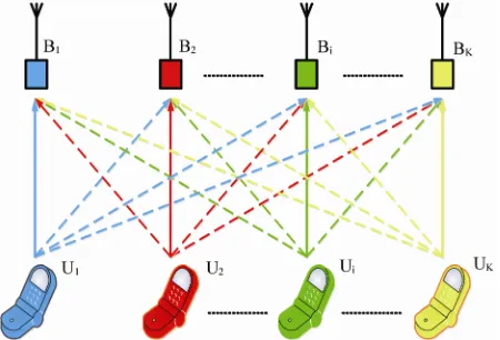
The research on achieving simultaneous transmissions and receptions has a long literature. In the [8], [9], the interference alignment [8] and zero forcing [9] methods are addressed in which, multiple transmitters jointly en- code and send their signals to intended receivers such that interfering signals are separated and eliminated [10]. In the IA in transmitters aligning matrices are applied to send the signals such that interfering signals at each re- ceiver lie in a subspace which is linearly independent of desired signal subspace [8]. Then, the zero forcing filter is applied to the received signal to eliminate interference signals and retain the desired signal. Consider a K-user interference channel consists of K transceivers pairs in which the transmitters 1 to K send their signals to

the receivers 1 to K. Each transmitter and receiver

is equipped with single antenna. As shown in Figure 1,

Figure 1. A K-user interference channel with K transmitters U1 to UK and K receivers B1 to BK.

each receiver only decodes the signal of its own trans- mitter and the signals of other transmitters are considered as interference. The desired and interference signals are shown by solid lines and dashed lines, respectively. It is assumed that the full channel state information is avail-able at every transmitter and receiver. The signal received by the i-th receiver can be expressed as

i Y

K

i ij i i ij i i i

j 1, j i 

 



Y H V S H V S Z  , 2,, K

S V

H

Z

12 2 13 3 1K K

i 1 (1)

where i represents the signal of transmitter i, i is

the aligning matrix for the i-th user, ij represents the

channel matrix from transmitter j to receiver i and i is

the additive white Gaussian noise with zero mean and unit variance. For perfect aligning of interferences of Transmitters 2 to K in Receiver 1, we should have

  

H V H V  H V

21 1 23 3 2K K

(2)

and in Receiver 2,

  

H V H V  H V

       

i1 1 i2 2 i i 1 i 1 i i 1 i 1

iK K

   

(3)

and in Receiver i

    



H V H V H V H V

H V

 

12 2 1j j

i1 1 ij j

0, j 1, 2

0, j 1, i, i 1

   

(4)

The Equations (2)-(4) can be shown as

     

H V H V

H V H V

i

W Y_i i1, 2,, K

(5)

By solving (5), aligning matrices are obtained and by aligning interference signals in each receiver, the desired signal subspace and interference signals subspace will be linearly independent. By applying the zero forcing filter to at each receiver, we get for .

1 K

i i i i ii i i i ij j j i

j 1, j i

  



where

i ij

W H Vj0 j i (7)

Thus,





i 1, 2,, K

NIA NIA

B

 

n B

i  i ii i i i i

Y W H V S W Z (8)

Figure 2 shows the IA solution for a 3-user interfer- ence channel. The desired and interference signals are presented by solid lines and dashed lines, respectively. The receiver of each user only needs to decode the signal of its own transmitter. By applying aligning matrices in transmitters, interference signals received at each re- ceiver align in a one-dimensional subspace and are line- arly independent of the desired signal subspace.

4. Proposed Method

We apply the IA technique to WSNs. Applying the IA to WSN is performed in three parts. First, we select those nodes which make use of the IA technique for trans- mission. In the second part, for network scheduling we color the conflict graph GC using a graph coloring algorithm. In the third part, network scheduling is ob- tained based on graph coloring. We assume the number of sensor nodes is N, the nodes which are using the IA is and the restare in the set . The number of an arbitrary set members such as is represented by

and parent of an arbitrary node such as C is represented by PA

 





 

n NIA (9)

4.1. Node Selection for Interference Alignment

In a WSN a single node can both gather and forward the packets. The nodes transmitting more packets, experience more strict congestion, which makes delay in packet transition to the BS. For a better performance, the IA technique is applied to the nodes with strict congestion.

Figure 2. IA solution for a 3-user interference channel.

Node selection has three stages. In the first stage, the forward degree for each node is computed. Forward degree for each node is equal to the number of nodes which forward their packets through that node over the routing tree. Figure 3 illustrates a network with the forward degree of nodes.

Then, nodes are ordered in a decreasing degree of forward. Assuming each node sends at least one packet at each transmission cycle, in the second stage, we choose the nodes with a high forward degree (nodes with degree more than 10 times of the minimum degree). In the third stage, we choose the sets of nodes among the selected nodes in the second stage which compose a multi-user interference channel with their parents. It means that the nodes of each set should be within the interference range of other set nodes and cannot transmit simultaneously without IA. Thus, an arbitrary set such as





S_a  nod_1a nod_2a  nod_Ka that composes a K-user interference channel, should have the following condi- tions:

1) Any two nodes of each set should have different parents.









PA nod PA nod i j  K i j (10)

2) The parent (receiver) of each node (transmitter) should be within the interference range of other set nodes (other transmitters).









d PA nod nod r i j  K i j (11)



where d i, j



3) Each node with its parent cannot be in the same set.









if nodiaSa then PA nodia Sa  i 1, 2,,K

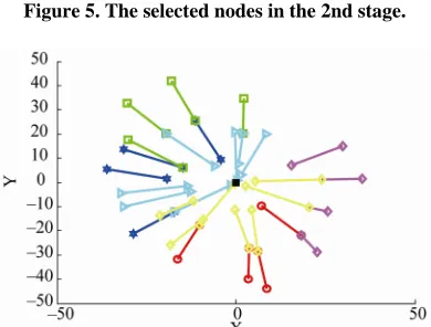
GC (12) For example, Figure 4 displays a WSN with 1000 nodes deployed in a circular area and the BS is located in the center of the circle. Figures 5 and 6 display selected nodes in the 2nd and 3rd stages, respectively. In this example, the number of sets are using the IA is six. The nodes of each set are shown in the same color.

4.2. Coloring of Network Graph

For transmission scheduling, first, we color the

   

 





GS GS

GS

GS

GS GS

GS

GS

NIA GC

NIA NIA

Figure 4. A WSN with 1000 nodes.

Figure 5. The selected nodes in the 2nd stage.

Figure 6. The selected nodes in the 3rd stage. the nodes using IA for transmission.

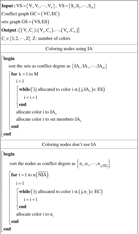
using a graph coloring algorithm. For this purpose each two nodes with different colors cannot transmit simulta- neously [5]. Coloring the network has two steps. In the first step, we color nodes using IA for transmission, i.e. nodes member of . In the second step, we color other nodes in the network, i.e. nodes member of . To assign color to the nodes of , weform the sets

graph with M . The

node i corresponds to all nodes at set i and two nodes i and

(13)

Then, the conflict degree for each node in the is obtained. The degree conflict of each node in the is equal to the number of connected edges. Then, the nodes in the are ordered in a decreasing degree of conflict and priority of coloring is given to the nodes with a more conflict degree. In coloring the , every two nodes conflict with each other have different colors. Thus, if two sets conflict with each other have different colors. Since all members of a set can transmit simultaneously, they have the same color. Then, the conflict degree for each node in the is obtained. The degree conflict of each node in the is equal to the number of con- nected edges. Then, the nodes in the are ordered in a decreasing degree of conflict and priority of coloring is given to the nodes with a more conflict degree. In coloring the , every two nodes conflict with each other have different colors. Thus, if two sets conflict with each other have different colors. Since all members of a set can transmit simultaneously, they have the same color.

For assigning color to the nodes , the degree conflict of each node in the is obtained. Then, nodes are ordered in a decreasing degree of conflict and the priority of color assignment is given to the nodes with a more conflict degree. As some colors were already assigned to the nodes , for assigning color to nodes the , conflict of each new node is examined with all nodes corresponding to each color. If there is no conflict, the color is assigned to the new node; otherwise, other colors should be examined.

Finally, if any color among available colors is not as- signed to the new node, a new color should be assigned. The coloring algorithm is given in Figure 7.

4.3. Scheduling Network

NIA

NIA NI

 ,S



A







S

S Sj are connected if there is an edge between a node at set i and any node at set j in the conflict graph of the original network. Thus, we have

The scheduling algorithm assigns one or more time slots to each node in the network for conflict-free communica- tion such that the delay in data collection is minimized. The network scheduling is obtained based on graph col- oring. A super slot in our scheduling algorithm is a set of sequential time slots such that each node having one packet or more at the beginning of the super slot sends at least one packet throughout the superslot. All of the nodes allocated to the same color can send at a time slot. The maximum number of slots in a superslot is the total number of colors utilized for coloring the network. After determining the nodes corresponding to the current time slot, as long as the resulting set is non-conflicting extra nodes allocated to other colors are added.

   

 

 

   

 

1 2 N

1 1 2 2

i

VS V , V , , V , VS

Conflict graph GC VC, EC

sets graph GS VS, ES

V , C , V , C , ,

C 1, 2, , Z Z : number of col

 



Input :

Output : 



 





1 2 M

N N S ,S , ,S

V , C

ors

   

Coloring nodes using IA

 

 



1 2 M

k

A , IA , , IA

t. j, IA ES

   k A



sort the sets as conflict degree as I k 1 to M

i 1

j allocated to color i s i i 1

allocate color i to IA allocate color i to set me

         begin for while end mbers I     _  _  _  _  _  _  _  _  _  _  _  _  _   end end

Coloring nodes don’t use IA

 





 

t

sort the nodes as conflict degree as

t 1 to n NIA

i 1

j allocated to color i st. i i 1

allocate color i to n

     _{ }  _  _{ }  _     _{ }     _      begin for while end end end           





1 2 n NIA

t n , n , , n

j, n EC

 



Figure 7. The coloring algorithm.

done once such that this part is not required for each data collection cycle. In other words, the node selection part loads no additional delay during the transmission. Other two parts of the proposed method have similar computa- tional complexity to the node-based and level-based scheduling algorithms.

5. Simulation Results

For evaluation of the proposed method, we use two met- rics; the delay and throughput. The delay is the time du- ration in which all packets generated by all nodes reach the BS. The throughput is the average rate of successful data delivery over the channel and it is measured in data packets per time slot. In simulations, the WSN consists of 1000 sensor nodes randomly distributed within a cir- cular area with radius of 100 units. The BS is located in the center of the circular area. The density of sensor nodes within the radius 100

and 100 is 2

2 is ₁ and between the

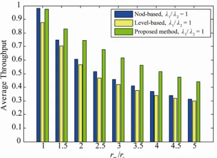
radius 100 2  . We use Dijkstra algo- rithm as shortest path routing to determine the routing tree rooted at the BS. The results presented here are the average performance of 100 different network realiza- tions. The results of simulation are compared to two TDMA scheduling algorithms, one node-based and the other level-based [5]. Figures 8 and 9 respectively dis- play the delay and average throughput of the proposed method in comparison with the TDMA scheduling algo- rithms versus  1 2 for rm rs2, respectively. As the simulations show, by using proposed method, the delay greatly reduces and throughput significantly increases.

This happens since in TDMA without using IA, the nodes which are within the interference range of each other cannot transmit simultaneously causing the delay to increase and throughput to decrease. In contrast, while IA is used, these nodes can transmit simultaneously. Hence, the number of concurrent transmissions increases leading the delay to decrease and throughput to increase. Also, the simulation results demonstrate that the per- formance of the proposed method depends on thenetwork topology. Figure 10 shows the percentage of perform- ance improvement (PPI) of the proposed method with respect to node-based and level-based algorithms versus

Figure 8. Comparison of delay of proposed method with those of node-based and level-based algorithms.

Figure 10. Percentage of delay performance improvement of proposed method with respect to node-based and level- based algorithms for different  _{1 2} ratios.

1 2

  . In Figure 10, by increasing the  1 2 ratio, the

PPI increases to a certain value and afterwards decreases. Therefore, for rm rs2, the proposed method presents a good PPI in topologies with the medium  1 2 ratios

and a lower PPI in the topologies with low and high

1 2

  ratios. These changes are due to dependency of the proposed method performance on two factors:

1) Interference degrees of selected nodes in 2nd stage

st2 : the interference degree for each node is the number of nodes interfere that with it. With increasing

st2, the number of nodes increases causing

improvement in proposed method performance because the proportion of packets transmitted by nodes to that of nodes increases.





deg NIA

NIA NIA





NIA diff diff

2) The difference between forward degrees of nodes and AA : With increasing AA

NIA , the

performance of the proposed method improves because the proportion of packets transmitted by nodes to that of nodes increases.

NIA NIA

With increasing  1 2 deg

diff

, st2 increases while

AA decreases. Up to a certain amount of  1 2

AA

iff 

, influence of st2 increment is predominant and after-

wards influence of decrement becomes predomi- nant.

deg d

Figures 11-13 show the impact of interference radius on performance of these methods. These figures show the delay of the methods versus rm rs for three ratios of

1 2

  as follows:

·   _{1 2} 1 9 , represents a topology in which the

density of packets is higher at the upper levels of the routing tree.

·   _{1 2} 1, represents a topology in which the density

of packets is equal throughout the network.

· _{1 2} 9 1

Figure 11. Comparison of the delay of proposed method with node-based and level-based algorithms versus r_m r_s for

   , represents a topology in which the

density of packets is higher at the lower levels of the routing tree.

Results show that with increasing the m s ratio, the delay is increased, because the number of the nodes

r r

1 2 1 9.

  

Figure 12. Comparison of the delay of proposed method with node-based and level-based algorithms versus r_m r_s for  _{1 2}1.

Figure 13. Comparison of the delay of proposed method with node-based and level-based algorithms versus r_m r_s for  _{1 2}9.

pect to the node-based algorithm versus m s. In Fi- gure 14, by increasing

r r m

r rs ratio for the topologies with the medium or high  1 2 ratios, the PPI increases

while for the topologies with low  1 2 ratios, the PPI

increases to a certain value and afterwards decreases. Figures 15-17 display the average throughput of these methods versus rm rs for three values of  1 2, res-

pectively. Simulation results show that the proposed me- thod performs better in topologies with the same ratio of

1

 and 2. This happens since in topologies with the

medium  1 2 ratio, both degst2 and diffAA is high

while in topologies with low  1 2 ratio, is

low and in topologies with high

st2

deg

1 2

  ratio, diffAA is

low.

6. Conclusion

We applied the IA technique to WSNs to reduce inter- ference effects. In this way, multiple transmitters jointly encode their signals to intended receivers such that interfering signals are separated and eliminated at each

Figure 14. Percentage of delay performance improvement of proposed method with respect to node-based algorithmfor different r_m r_s ratios.

Figure 15. Comparison of the throughput of proposed me- thod with node-based and level-based algorithms versus

m s

r r for  _{1 2}1 9.

Figure 16. Comparison of the throughput of proposed me- thod with node-based and level-based algorithms versus

m s

r r for  1 21.

Figure 17. Comparison of the throughput of proposed me- thod with node-based and level-based algorithms versus

m s

r r for  1 29.

receiver. By applying the proposed methodto WSNs, delay and throughput performances significantly improve. The performance of the proposed method depends on the network topology. Compared to the topologies with low and high 1 2 ratios, in the topologies with the me-

dium  1 2 ratios, the percentage of performance im-

provement in the proposed algorithm is more.

REFERENCES

[1] H. Choi, J. Wang and E. A. Hughes, “Scheduling for In- formation Gathering on Sensor Network,” Wireless Net-works, Vol. 15, No. 1, 2009, pp. 127-140.

doi:10.1007/s11276-007-0050-9

[2] J. Zheng and A. Jamalipour, “Wireless Sensor Networks: A Networking Perspective,” John Wiley & Sons, Inc., Hoboken, 2009.

Per-vasive Computing and Communications, Hong Kong, 17-21 March 2008, pp. 264-268.

[4] G. Lu, B. Krishnamachari and C. S. Raghavendra, “An Adaptive Energy-Efficient and Low-Latency MAC for Data Gathering in Wireless Sensor Networks,” Proceed-ings of the 18th International Conference of the IEEE IPDPS, Santa Fe, 26-30 April 2004, pp. 224-231.

[5] S. C. Ergen and P. Varaiya, “Tdma Scheduling Algo-rithms for Wireless Sensor Networks,” Wireless Networks, Vol. 16, No. 4, 2010, pp. 985-997.

doi:10.1007/s11276-009-0183-0

[6] W. Wang, Y. Wang, X. Y. Li, W. Z. Song and O. Frieder, “Efficient Interference-Aware TDMA Link Scheduling for Static Wireless Networks,” Proceedings of the 12th Annual International Conference of the ACM Mobile Computing and Networking, Los Angeles, 23-26

Sep-tember 2006, pp. 262-273.

[7] P. Gupta and P. Kumar, “The Capacity of Wireless Net-works,” IEEE Transactions on Information Theory, Vol. 46, No. 2, 2000, pp. 388-404. doi:10.1109/18.825799

[8] V. Cadambe and S. Jafar, “Interference Alignment and the Degrees of Freedom of the K User Interference Chan- nel,” IEEE Transactions on Information Theory, Vol. 54, No. 8, 2008, pp. 3425-3441.

doi:10.1109/TIT.2008.926344

[9] D. Tse and P. Viswanath, “Fundamentals of Wireless Com- munication,” Cambridge University Press, Cambridge, 2005.