Guided and Direct Wave Evaluation of Controlled Source
Electromagnetic Survey Using Finite Element Method
Noorhana Yahya1, Majid Niaz Akhtar2, Nadeem Nasir2, Muhammad Kashif2, Afza Shafie1, Hasnah Mohd Zaid1
1
Fundamental and Applied Sciences Department, Bandar Seri Iskandar, Tronoh, Malaysia; 2Electrical and Electronic Engineering Department, Universiti Teknologi PETRONAS, Bandar Seri Iskandar, Tronoh, Malaysia.
Email: [email protected]
Received January 15th,2012; revised February 14th, 2012; accepted February 24th, 2012
ABSTRACT
Deep target hydrocarbon detection is still challenging and expensive. Direct hydrocarbon indicators (DHIs) in seismic data do not correspond to economical hydrocarbon exploration. Due to unreliability in seismic data for the detection of DHIs, new methods have been investigated. Marine controlled source electromagnet (MCSEM) or Sea bed logging (SBL) is new method for the detection of deep target hydrocarbon reservoir. Sea bed logging has also the potential to reduce the risks of DHIs in deep sea environment. Modelling of real sea environment helps to reduce the further risks before drilling the oil wells. 3D electromagnetic (EM) modelling of seabed logging requires more accurate methods for the detection of hydrocarbon reservoir. Finite element method (FEM) is chosen for the modelling of seabed logging to get more precise EM response from hydrocarbon reservoir below 4000 m from seabed. FEM allows to investigate the total electric and magnetic fields instead of scattered electric and magnetic fields, which shows accurate and precise resistivity contrast below the seabed. From the modelling results, It was investigated that Hz field shows higher magni- tude with 342% than the Ex field. It was observed that 0.125 Hz frequency can be able to show better resistivity contrast of Hz field (31.30%) and Ex field (16.49%) at target depth of 1000 m below seafloor for our proposed model. Hz and Ex field delineation was found to decrease as target depth increased from 1000 m to 4000 m. At the target depth of 4000 m, no field delineation response was seen from the current electromagnetic (EM) antenna used by the industry. New EM antenna has been used to see the EM response for deep target hydrocarbon detection. It was investigated that novel EM antenna shows better delineation at 4000 m target depth for Ex and Hz field up to 10.3% and 15.1% respectively. Novel EM antenna also shows better Hz phase response (128.4%) than the Ex phase response (38.3%) at the target depth of 4000 m below the seafloor.
Keywords: Sea Bed Logging; Controlled Source Electromagnetic (CSEM); Electromagnetic (EM) Antenna and Finite Element Method
1. Introduction
Marine controlled source electromagnetic (MCSEM) surveying has become promising tool for remotely de- tecting, characterizing and mapping offshore hydrocar- bon reservoirs. MCSEM survey has an advantage over seismic method due to low cost, accurate and economic for shallow as well as deep target [1,2]. MCSEM method also referred as seabed logging uses EM transmitter for the transmission of EM waves into marine environment. EM receivers are placed on seabed to record the EM waves after reflected, refracted and guided back from different resistive layers such as sediments and hydro- carbon. Low frequency EM waves ranges from (0.01 to 10 Hz) has been used for the detection of hydrocarbon reservoir situated at different depths below seabed [3,4].
to current flowing along the antenna. Higher the Q values can give higher efficiency of power. It was also observed that hysteresis losses and eddy current losses increases as the frequency increases [5,6]. Magnitude of EM waves increased by using magnetic feeders on the antenna was also investigated [7,8]. It was found that magnitude of EM waves can be increased up to 243% using magnetic feeders on the antenna in lab scale environment [9]. Electric field response from different gas hydrate models were investigated by exciting horizontal electric dipole source. MCSEM method requires modelling tools for the characterizing, mapping and detection of hydrocarbon reservoir. Different numerical modelling tools such as Finite element method (FEM), Finite difference method (FDM), Transmission line matrix (TLM) method, Method of moment (MOM), Boundary element method (BEM) etc. [10]. Finite element method is a versatile technique to find approximate solution of partial differential equations (PDE) as well as integral equations. Finite element method uses Maxwell’s equations for the solution of electro- magnetic (EM) problems. FEM method investigated de- tailed visualization of resistive layers in MCSEM envi- ronment [11]. The effect of different values of transmit- ting frequency from the source, distance between the source and the seabed, water depth and thickness of over- burden layer was observed during the study [12].
2. Theoretical Background
Finite element method has been used to solve CSEM problems. Maxwell’s equations were solved using coulomb gauged EM potentials where as sparse system of linear equations was solved by using Quasi minimal residual method. It was also investigated that finite element is a general method and can be easily applied for CSEM modelling [13].
In finite element method (FEM), Galerkin method mi- nimizes the errors over the entire volume of the proposed model. It was studied that FEM has not required quasi static approximation. FEM can be easily applied to the complex and homogenous structures due to Galerkin approximation [14]. FEM uses the process of discre- tization of the region by creating meshes. Meshing is used to subdivide a large geometry into a number of non overlapping sub regions. It is necessary to discretize physical structure regular or irregular into finite number of degrees of freedom. Finite element method (FEM) can be easily applied to arbitrarily geological structures due to unstructured meshes. Finite element (FE) modelling results show less than 1% error as compared to Finite difference time domain (FDTD) and Method of moment (MoM) etc. [15]. Modelling of geophysical electro- magnetic methods by finite element has been discussed by [16,17]. The electric and magnetic field differential equations for the solution of EM problem are
2 0 2 2 0 2 0 0 x x z z Ei y E
y
H i y H
y (1)
In finite element method, explicit specification of approximate electric field is
1 1
N
x i i
i N
z i i
i
E y E y
E y E y
(2) where,
i y are the basis functions, whereas Ei and Hi
are the coefficients of approximate electric and magnetic field in this expression.
1 1 1 1 , , 0 otherwisei i i i i
i i i i i
y y y y y y y
y y y y y y y y
i1
(3)
Approximate electric field is linear between each pair of nodes where as it has continues value at each node. For the solution of true electric field, the approximate electric and magnetic fields are
2 0 2 1 0 N i i i iE i y R
y
(4)and
2 0 2 1 0 N i i i iH i y R
y
(5)where,
R is residual due to applied electric or magnetic field,
ψj is weight functions. The electric field equation is
2 0 2 1 0 N ii j j i j
i
E i y
y
R
(6)1 1 1
2
0 2
1
d d
N N N
y y y
N
i
i j j j
i y y i y
E y i y R
y
dy 0
(7)R is orthogonal to weight function j
1 d 0 N y j y R y
(8)to solve electromagnetic problem by FEM. In Galerkin method, basis functions are used as weight functions, which make square system with N equations in N un- knowns. 1 1 2 0 2 1 d d N N y y N i
i j j i
i y y
E y i y
y
0 (9)1
1 1
1 1
1
2
2d d
yi i i y y y j i i j y y y y
y y y
y i j
(10)As basis functions are continues, then using Galerkin method, weight function will be continues.
1 1 1 1 2 2d i i y y j i j y y y y y y
idy (11)1 1 0 1 d d N N y y N j i
j i i
i y y
y i y E
y y
0 (12)Similarly, the magnetic field equation can be written as
1 1 0 1 d d N N y y N j i
j i i
i y y
y i y H
y y
0 (13)
0
0
L i S r
L i S r
E H (14)
E and H are the vectors containing coefficient for each node in finite element (FE) expression for approximate electric and magnetic fields,
1 1
d d
N N
y y
j i
ji ji j i
y y y y y y
L SL and S are NN matrices. By solving these matrices, electric field can be solved straight forward for 1D electromagnetic (EM) problem. For EM problems a large number of equations with many matrices need to be solved. Different commercial soft wares have been used to study the EM geological problems.
The current study is about the modelling of real seabed environment by using conventional EM antenna and novel EM antenna for deep target hydrocarbon detection. Comsol multiphysics based on finite element method have been used to solve deep target problem. All field components (Ex, Ey and Ez) and (Hx, Hy and Hz) with and without hydrocarbon were also compared during the study. Magnitude of E field and H field response from resistive layers was also compared during the study. Section 3 will describe about the methodology adapted to achieve the objectives. In Section 4, results obtained using conventional and new Electromagnetic antenna will be discussed in detail.
3. Methodology
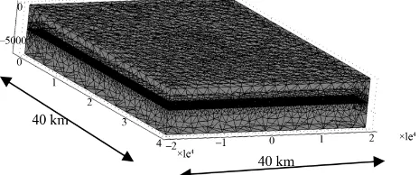
Finite element method (FEM) was used to detect hydro- carbon below several hundred of meters from seabed. (Comsol Multiphysics-3.5a) based on finite element method (FEM) was used to simulate area of the seabed model contains 40 × 40 km. Seabed model with air thickness 500 m, sea water depth 1000 m, overburden 1000 m, hydrocarbon thickness 100 m and under burden thickness 3500 m was constructed. 0.125 Hz frequency with 1250 A current was used at the transmitter. Different models were simulated after increasing target depth of 500 m from 1000 to 400 m below seafloor. The position of the antenna was 30 m above the seafloor. The length of the antenna was kept 270 m. The frequency was decreased from 0.125 Hz to 0.0625 Hz and current was increased from 1250 A to 7200 A at 4000 m target depth. New EM antenna with magnetic feeders was used in our proposed model to get better delineation response at target depth of 4000 m. Triangular meshes with free mesh parameter of 1.0e–3 were selected. Refined meshes were also used to get more precise and accurate results. Sub domain set- tings with conductivity and relative permittivity of air, sea water, under burden, overburden and hydrocarbon were adjusted as given in Table1. Boundary conditions were adjusted on the proposed seabed model to get the electric and magnetic response. Partial differential equa- tions for magnetic and electric fields in the wave number domain were also used to get total electric and magnetic field response with and without hydrocarbon. Figure1
[image:3.595.79.288.140.214.2]shows schematic diagram of seabed model with trans- mitter and receivers on the seabed.
Table 1. Relative permittivity, conductivity values of air, sea water and hydrocarbon.
Air Sea water Under-burden /Overburden
Hydrocarbon (Oil)
r 1.006 80 30 4
1.0e–13 3 1.5 0.001
[image:3.595.309.539.503.719.2]4. Results and Discussions
Finite element method is used to simulate the CSEM experiment on our proposed seabed model. Figure 2
shows finite element method applied on proposed seabed model. The finite element generates meshes on the pro- posed model to get the EM response from the marine environment such as seawater, overburden, under burden and hydrocarbon etc. Finite element creates refined meshes with thousands of interconnecting nodes. More refined meshes at the transmitter and receiver especially for small transmitter and receiver offsets were used to get more precise and accurate results [18]. Figures 3(a)-(c)
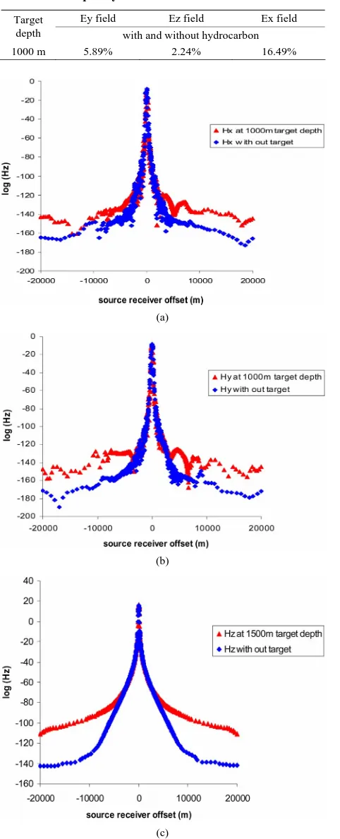
show Ey, Ez and Ex field response with and without hydrocarbon located at 1000 m below the seafloor respectively. It was found that Ey and Ez components have no ability for the detection of hydrocarbon in our proposed seabed model. It was observed that Ex component gives better response in terms of magnitude and delineation as compared to other two components Ey and Ez. Ex component gave smooth and better response due to propagation of EM waves in y-direction from inline orientation of EM transmitter. Table 2 shows the comparison of Ey, Ez and Ex field components with and without HC at target depth of 1000 m below seabed.
Figures 4(a)-(c) show Hx, Hy and Hz field response with and without hydrocarbon located at 1000 m below the seafloor respectively. It was found that Hx and Hy components have no ability for the detection of hydro- carbon in our proposed seabed model. It was observed that Hz component gives better response in terms of magnitude and delineation as compared to other two components Hy and Hx. Hz component gave smooth and better response due to propagation of EM waves in y-direction from inline orientation of EM transmitter.
[image:4.595.57.289.610.707.2]Table3 shows the comparison of Hx, Hy and Hz field components with and without HC at target depth of 1000 m below seabed. It can be seen that Ex and Hz field components show delineation response than all the other components, where as Hz field gave better delineation (31.3%) than Ex field component (16.4%) at target depth of 1000 m below seabed. It was also investigated that Hz field gave higher magnitude with better delineation as compared to Ex field component.
Figure 2. Seabed logging model with meshes generated by FEM.
Figures 5(a)-(g) show normalized E field response with and without hydrocarbon located at 1000 m, 1500 m, 2000 m, 2500 m, 3000 m, 3500 m and 4000 m below the seafloor respectively. It was found that normalized E
(a)
(b)
(c)
Table 2. Ex, Ey and Ez components at 1000 m target depth at 0.125 Hz frequency with 1250 A current at transmitter.
Ey field Ez field Ex field Target
depth with and without hydrocarbon
1000 m 5.89% 2.24% 16.49%
(a)
(b)
(c)
Figure 4. Log (H) components vs source receiver offset (a) Hx component; (b) Hy component; (c) Hz component with and without HC at 1000 m target depth from seabed.
Table 3. Hx, Hy and Hz components at 1000 m target depth at 0.125 Hz frequency with 1250 A current at transmitter.
Hy field Hz field Hx field Target
depth with and without hydrocarbon
1000 m 5.68% 7.16% 31.3%
(a)
(b)
[image:5.595.57.298.105.699.2](d)
(e)
(f)
(g)
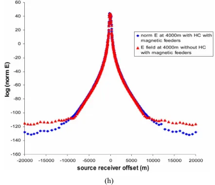
[image:6.595.311.532.86.277.2](h)
Figure 5. Magnitude of H field verses source receiver offset with and without HC at (a) 1000 m; (b) 1500 m; (c) 2000 m; (d) 2500 m; (e) 3000 m; (f) 3500 m; (g) 4000 m; at 0.125 Hz; (h) with 9 magnetic feeders using finite element method.
field at the offset decreased as the depth increased from 1000 m to 4000 m. It can be seen that at target depth of 1000 m normalized E field response was 16.49% but as the depth increased up to 4000 m, E field response de- creased up to (1.10%). Comparison of percentage of normalized E field with and without hydrocarbon with different target depths are given in Table4. It was found that at 4000 m target depth with 0.125 Hz frequency and 1250 A current, it was not possible to see the hydrocar- bon. The frequency was decreased from 0.125 Hz to 0.0625 Hz at 1250 A; the delineation response of 2.84% was investigated. The increase of current from 1250 A to 7200 A at target depth of 4000 m target depth, we get normalized E field response up to 2.45% with and with- out HC. The decrease in frequency from 0.125 Hz to 0.0625 Hz gives us delineation but resolution will be not good at the low frequency. Novel EM antenna with 3, 6 and 9 magnetic feeders was used for deep hydrocarbon survey. EM antenna with 9 magnetic feeders has shown promising results for the direct hydrocarbon detection below 4000 m from the seabed (Figure 5(h)). It was in- vestigated that by using 9 magnetic feeders at the antenna, we can get better delineation up to 10.3% (Table4).
Table 4. Comparison of percentage of magnitude of Ex and Hz field and phase with and without hydrocarbon at dif- ferent target depth.
Ex field Ex phase Hz field Hz phase Target
depth (m)
Frequency (Hz)
Current
(A) with and without hydrocarbon
1000 0.1250 1250 16.4 78.7 31.3 164.3
1500 0.1250 1250 10.4 42.1 16.3 139.5
2000 0.1250 1250 6.74 26.6 9.74 123.1
2500 0.1250 1250 5.15 17.5 7.73 48.7
3000 0.1250 1250 3.58 7.04 5.12 18.0
3500 0.1250 1250 2.94 5.03 3.46 7.95
4000 0.1250 1250 1.10 3.64 2.54 4.04
4000 0.0625 1250 2.84 3.27 3.82 4.01
(a)
(b)
(c)
[image:7.595.56.288.113.734.2](d)
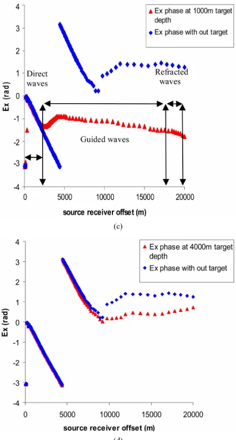
Figure 6. Direct, guided and reflected waves behavior of Ex field at (a) 1000 m target depth and (b) 4000 m target depth and Ex phase at (c) 1000 m target depth and (d) 4000 m tar- get depth with and without HC with and without HC using finite element method.
was seen due to shallow target, where as the target depth increases the guided response decreases. At the target depth of 4000 m, no guided response was seen (Figure 6(b)). New EM antenna at 4000 m target depth gives guided response of EM waves with better delineation up to 10.3%. It was investigated that the guided wave re- sponse is greater and can be comparable to the target depth at 1500 m from seafloor.
provides changes in resistivity which can be helpful for the verification of the MVO results. Phase with the source receiver offset are also investigated Figures6(c) and (d). It was investigated that phase at 1000 m gave 78.7% delinea- tion response where as at 4000 m target depth 3.64%
Figures6(c) and (d). It was observed that as target depth increased from 1000 m to 4000 m, the electromagnetic signal attenuates rapidly [1]. Table 5 shows the com- parison between Ex phase with source receiver offset with and without hydrocarbon at target depth changes from 1000 m to 4000 m. It was found that Ex phase shows better delineation (38.3%) with and without HC by using 9 magnetic feeders at EM antenna (Table5).
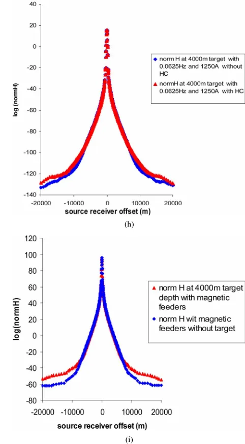
Figures 7(a)-(g) show normalized H field response with and without hydrocarbon located at 1000 m, 1500 m, 2000 m, 2500 m, 3000 m, 3500 m and 4000 m below the seafloor respectively. It was found that normalized H field at the offset decreased as the depth increased from 1000 m to 4000 m. It can be seen that at target depth of 1000 m normalized H field response was 31.3% but as the depth increased up to 4000 m, H field response decreased up to (2.54%). Comparison of percentage of normalized E field with and without hydrocarbon with different tar- get depths are given in Table4. It was found that at 4000 m target depth with 0.125 Hz frequency and 1250 A cur- rent, it was not possible to see the hydrocarbon. The fre- quency was decreased from 0.125 Hz to 0.0625 Hz at 1250 A; the delineation response of 3.82% was investi- gated. The decrease in frequency from 0.125 Hz to 0.0625 Hz gives us delineation but resolution will be not good at the low frequency. Novel EM antenna with 3, 6 and 9 magnetic feeders was used for deep hydrocarbon survey. EM antenna with 9 magnetic feeders has shown promising results for the direct hydrocarbon detection below 4000m from the seabed (Figure 7(h)). It was in- vestigated that by using 9 magnetic feeders at the antenna, we can get better delineation up to 15.1% (Table4).
(a)
(b)
(c)
(e)
(f)
(g)
(h)
[image:9.595.296.537.85.522.2](i)
Figure 7. Magnitude of Hz phase verses source receiver offset with and without HC at (a) 1000 m; (b) 1500 m; (c) 2000 m; (d) 2500 m; (e) 3000 m; (f) 3500 m; (g) 4000 m at 0.125 Hz; (h) 4000 m target at 0.0625 and (i) with 9 mag- netic feeders using finite element method.
(a)
(b)
(c)
[image:10.595.57.289.80.734.2](d)
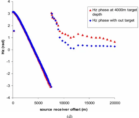
Figure 8. Direct, guided and reflected waves behavior of Hz field at (a) 1000 m target depth and (b) 4000 m target depth and Hz phase at (c) 1000 m target depth and (d) 4000 m target depth with and without HC using finite element method.
At the target depth of 4000 m, no guided response was seen (Figure 8(b)). New EM antenna at 4000 m target depth gives guided response of EM waves with better delineation up to 15.1%. It was investigated that the guided wave response is greater and can be comparable to the target depth at 1500 m from seafloor.
Phase with the source receiver offset are also investi- gated Figures 8(c) and (d). It was observed that per- centage difference in phase also decreased as the target depth increased from 1000 m to 4000 m. It was investi- gated that phase at 1000 m gave 164.3% delineation re- sponse where as at 4000 m target depth 4.32% (Figures 8(c) and (d)). Table5 shows the comparison between Hz phase with source receiver offset with and without hy- drocarbon at target depth changes from 1000 m to 4000 m. It was found that Hz phase shows better delineation (128.4%) with and without HC by using 9 magnetic feeders at EM antenna (Table5).
[image:10.595.306.540.86.284.2]observed that as the target depth increased the delinea- tion response decreased. This is due to the week signals from hydrocarbon detected by the receivers at the sea- floor. It is highly needed to increase the strength of the antenna. In this research work, the antenna was modified using magnetic feeders (prepared from novel magnetic materials). The magnetic feeders were used to excite the TM components such as H , Ez, and E. When the magnetic feeders were used on the antenna (conductor), the magnetic flux energy will be transferred from mag- netic feeders to the current flowing along the antenna conductor. Higher values of Q gave better efficiency of the power which is delivered to the antenna current. When toroidal core is excited by using AC source then due to magnetization magnetic field H generated. Mag- netic field “H” generated around the full loop constraint entire field to the core material (Biot and Savarts law). Electric field is concentrated at the middle of the mag- netic feeder due to the trapped magnetic field inside the circular loop which is due to the Maxwell’s relations (E is perpendicular to the H field). When a conductor is placed at the point of concentrated electric field, a large amount of current is induced in the wire conductor antenna [5].
The magnetic feeders play an important role for the excitation of electromagnetic antenna. The antenna with magnetic feeders has been used for deep target survey. It has been investigated that by using 3 magnetic feeders it is possible to detect the hydrocarbon reservoir with E and H field delineation response up to 3.89% and 4.25% re- spectively. This is still risking factor to drill the well for the industry due to high cost in oil well drilling. The numbers of magnetic feeders are increased from 3 to 6 magnetic feeders and it has been investigated that de- lineation response increased from 5.41% to 7.68% for E and H field respectively. The delineation responses gave very close values for Ex and Hz fields for our new EM antenna with 9 magnetic feeders when the target was at 1500 m which is in accord with the current industrial practice. In comparison of the E and H field responses, it can be seen that the H field and phase gave better de- lineation responses with a higher magnitude which was due to the amplitude of the magnetic field decreasing approximately by 1/R2
[image:11.595.307.540.122.231.2], whereas the electric field ampli- tude decreased by 1/R3 [19]. Table5 also shows the Ex, Hz field and phase response at the target depth of 4000 m by using 12 magnetic feeders at the EM antenna. The delineation response decreased due to the threshold val- ues of the increased magnetic feeders at the EM antenna. The simulation results of antenna with 9 magnetic feed- ers show good results for E and H field delineation re- sponse (10.3% and 15.1%) at 4000 m target depth. The results are in accord with the E and H field response at 1500 m target depth for our proposed model and with current industrial antenna used for seabed logging survey. EM antenna with magnetic feeders has an ability to detect
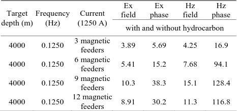
Table 5. Comparison of Ex and Hz field and phase with and without hydrocarbon at 4000 m target depth with 3, 6, 9 and 12 magnetic feeders.
Ex field
Ex phase
Hz field
Hz phase Target
depth (m)
Frequency (Hz)
Current (1250 A)
with and without hydrocarbon
4000 0.1250 3 magnetic feeders 3.89 5.69 4.25 16.9
4000 0.1250 6 magnetic
feeders 5.41 15.2 7.68 94.1
4000 0.1250 9 magnetic
feeders 10.3 38.3 15.1 128.4
4000 0.1250 12 magnetic
feeders 8.91 30.2 11.3 116.8
hydrocarbon in deep water and deep target environment due to its better stability.
5. Conclusion
Novel EM antenna was successfully used for the deep target hydrocarbon detection 4000 m below seabed. It was observed that 0.125 Hz frequency can be able to show better resistivity contrast of Hz field (31.3%) and E field (16.4%) for our proposed model. It was analyzed that field response delineation decreases as target depth increases from 1000 m to 4000 m. From the results, it was observed that at the target depth of 4000 m below seabed no H field delineation response was seen from the current used antenna by the industry. New EM antenna has been used to see the EM response for deep target detection. It was investigated that novel EM antenna shows better delineation for E and H field up to 10.3% and 15.1% respectively with and without hydrocarbon. New EM antenna has also an ability to show better Hz phase delineation response (128.4%) than the Ex phase response (38.3%). 3D FEM can provide helpful informa- tion for the development of instruments used for the de- tection of hydrocarbon in CSEM environment.
REFERENCES
[1] S. Ellingsrud, T. Eidesmo and S. Johansen, “Remote Sensing of Hydrocarbon Layers by Seabed Logging (SBL): Results from a Cruise Offshore Angola,” The Leading Edge, Vol. 21, No. 10, 2002, pp. 972-982. doi:10.1190/1.1518433 [2] F. N. Kong, H. Weterdahl, S. Ellingsrud, T. Eidesmo and
S. Johansen, “Seabed Logging: A Possible Direct Hydro- carbon Indicator for Deepsea Prospects Using EM Energy,” Oil and Gas Journal, Vol. 100, No. 19, 2002, pp. 30-38. [3] M. N. Akhtar, N. Yahya, H. Daud, A. Shafie, H. M. Zaid,
M. Kashif and N. Nasir, “Development of EM Wave Guide Amplifier Potentially Used for Sea Bed Logging,” Journal of Applied Science, Vol. 11, No. 7, 2011, pp. 1361-1365. doi:10.3923/jas.2011.1361.1365
Journal of Applied Science, Vol. 11, No. 7, 2011, pp. 1309-1314.doi:10.3923/jas.2011.1309.1314
[5] F. N. Kong, H. Westerdahl and F. Antonsen, “Excitation of a Long Wire Antenna-Antennas from 200 MHz to 1 Hz,” Tenth International Conference on Ground Penetrating Radar, Delft, 21-24 June 2004, pp. 137-140.
[6] N. Yahya and T. Zhu, “Development of Y3Fe5O12 Nano- Magnetic Feeder for Em Source of an Intelligent Horizontal Twin Dipoles,” American Institute of Physics, Vol. 1136, 2009, pp. 269-276.
[7] M. N. Akhtar, N. Yahya and N. Nasir, “Novel EM Antenna Based on Y3Fe5O12 Magnetic Feeders for Improved MVO,” Electronics, Communications and Photonics Conference, 2011 Saudi International, 24-26 April 2011, pp. 1-6.
[8] N. Yahya, M. N. Akhtar, N. Nasir, A. Shafie, M. S. Jabeli and K. Koziol, “CNT Fibres/Aluminium-NiZnFe2O4 Based EM Transmitter for Improved Magnitude vs Offset (MVO) in a Scaled Marine Environment,” Journal of Nanoscience and Nanotechonology, Vol. 11, No. 7, 2011, pp. 1-7. [9] M. N. Akhtar, N. Yahya, K. Koziol and N. Nasir,
“Synthesis and Characterizations of Ni0.8Zn0.2Fe2O4- MWCNTs Composites for Their Application in Sea Bed Logging,” Ceramics International, Vol. 37, No. 8, 2011, pp. 3237-3245.doi:10.1016/j.ceramint.2011.05.113 [10] N. O. Sadiku, “Numerical Methods in Electromagnetics,”
2nd Edition, Mathew, Boca Raton, London, New York, Washington DC, 2001.
[11] M. Deng, W. B. Wei, W. B. Zhang, Y. Sheng, Y. J. Li and M. Wang, “Electric Field Responses of Different Gas Hydrate Models Excited by a Horizontal Electric Dipole Source with Changing Arrangements,” Petroleum Explora- tion & Development, Vol. 37, No. 4, 2010, pp. 438-442.
[12] E. A. Badea, M. E. Everett, G. A. Newman and O. Biro, “Finite-Element Analysis of Controlled-Source Electro- magnetic Induction Using Coulomb Gauged Potentials,” Geophysics, Vol. 66, No. 3, 2001, pp. 786-799.
doi:10.1190/1.1444968
[13] F. Sugeng, A. Raiche and G. Wilson, “An Efficient Compact Finite-Element Modelling Method for the Practical 3D Inversion of Electromagnetic Data from High Contrast Complex Structures,” IAGA WG 1, 2 onElectromagnetic Induction in Earth, Spain, September 2006, pp. 17-23. [14] J. Park, T. I. Bjornara, H. Westerdahl and E. Gonzalez,
“On Boundary Conditions for CSEM Finite Element Modeling. I,” Proceedings of the Comsol Conference, Hannover, 2008, pp. 1-4.
[15] F. N. Kong, S. E. Johnstad, T. Røsten and H. Westerdahl, “A 2.5D Finite Element Modeling Method for Marine CSEM Modeling in Stratified Anisotropic Media,” Geophysics, Vol. 73, No. 1, 2008, pp. F9-F19.
doi:10.1190/1.2819691
[16] C. G. Farquharson, “Numerical Modeling for Geophysical Electromagnetic Methods,” Memorial University of Newfoundland, St. Johns, 2009.
[17] D. S. Parasins, “Principles of Applied Geophysics,” 5th Edition, Chapman & Hall, London, 1997.
[18] J. D. King, “Using a 3D Finite Element Forward Modelling Code to Analyze Resisitive Structures with Controlled Source Electromagnetics in a Marine Environment,” Master’s Thesis, Texas A&M University, College Station, 2004.