Time Representation in Economics
Stefano Bosi, Lionel Ragot
EPEE (Centre d’Etudes des Politiques Economiques de l’Université d’Evry), University of Evry, Evry, France Email: {stefano.bosi, lionel.ragot}@univ-evry.fr
Received October 31, 2011; revised November 27, 2011; accepted December 5, 2011
ABSTRACT
In this paper, we study general polynomial discretizations in backward and forward looking, and the preservation of stability properties. We apply these results to the Ramsey model [1]. Its discrete-time version is a hybrid discretizations of a backward-looking budget constraint and a forward-looking Euler equation. Saddle-path stability is a robust property under discretization.
Keywords: Discretization; Growth
1. Discretizations
Continuous-time systems can be approximated by discrete- time systems. In the spirit of Krivine, Lesne and Treiner [2], we bridge continuous and discrete-time dynamics through general polynomial discretizations.
Discretizations can differ according to the step, the order and the direction of discretization. The step gives the length of the period in discrete time. The order is that of the Taylor expansion of a continuous-time model. The direction depends on the backward or forward-looking nature of this Taylor expansion. A hybrid discretization mixes backward and forward-looking approximations.
We want to show that the steady state is invariant to the step, the order and the direction of discretization and its continuous-time stability properties (sink, saddle, source) are preserved under a sufficiently small discretization step in any case (backward, forward or hybrid).
Instead of considering a continuous variable t and the corresponding position x t
determined by an m-dimen- sional system of ordinary differential equations:
= ,
x f x where 0
,
fC jointly with the initial condition let us pick up a regular sequence of time val-ues:
0 0
x x ,
tn n=0 =
nh n=0
,
where h is a (possibly small) positive constant (discreti- zation step), and the associated values:
=
n n
x x t x nh .
The path from xn to xn1 can be reconstructed
component by component through an appropriate inte- gration of x= f x
m
x
. Focusing on the ith component of
the vector , we can integrate the time derivative
on the right or on the left to obtain, respectively,
1
= =
1
=0 =0
=
= d = d
=
= d = d
in in i i
nh nh
i i
nh h nh h
in in i i
nh h nh h
i i
nh nh
x x x nh h x nh
x t f x t t
x x x nh h x nh
x t f x t t
with i= 1,,m. Defining
d
d
nh
i nh i
nh h
i nh i
f x t t
f x t t
we get i
h =xin1xin=i
0
.A discretization is an approximation of i
( i
) through a simpler function evaluated at =h( = 0 ). The Euler-Taylor discretization is a polynomial approximation. Assuming that f Cq1 and consider- ing the qth order polynomial, we obtain a backward or a forward-looking discretization:
1
=0
=1
0
= 0
!
0
= 0
!
p q
p
in in i i
p p q
p i p
h
x x h
p
h p
(1)
1
=0
=1
0
= 0
!
0 =
!
p q
p
in in i i
p p q
p i p
h
x x h
p
h
h p
(2)
Setting , we obtain from (1) and (2) a first-order discretization:
= 1
q
1
1
= 0 0
= 0
= 0 0
= 0
'
in in i i
i
'
in in i i
i
x x h h
hf x nh
x x h h
h f x nh h
that is
1
in in i n
x x hf x (3)
1
in in i n x x hf x1
n
(4)
where the subscript i denotes the ith component of the vector.
Equation (3) (respectively, (4)) constitutes a backward- looking (forward-looking) discretization, because the varia- tion xn1x depends on the past value xn (future value
1
n
x ) on the right-hand side. Equation (3) is the classical Euler discretization. In economics, forward-looking dis- cretizations are of interest because agents behave ac- cording to their expectations.
The sequences
xn are approximations of the truesequence
x nh
, exact solution to system x= f x
: the smaller h, the more accurate the representation.Higher-order discretizations are also possible. Let us dis- cretize the continuous-time dynamical system x= f x
with fC1 by second-order Taylor polynomials, that is approximate the ith component of xn1 ith a quadratic
form. Using (1) and (2), we obtain in backward and for-ward-looking, respectively:
w
2
1
=1
2
1 1 1
=1 1
2
2
m
i
in in i n j n n
j jn
m
i
in in i n j n n
j jn
f h
x x hf x f x x
x
f h
x x hf x f x x
x
1where the subscript i denotes the ith component of the vector.
If f is an analytic function, infinite-order backward or forward discretizations converge exactly to xn1xn and (1) and (2) now hold with equality:
1
=1
=1
0
= 0
!
0 =
! p
p
in in i
p
p p i p
h
x x
p
h
h p
In this case, the Taylor polynomials become a conver- gent series and the discretized dynamics represent ex- actly the continuous-time system whatever the step h.
In general, a discretization is a closer approximation of a continuous-time system when the step h is smaller or the order of discretization q higher. The dynamic proper-
ties of a continuous-time system can be preserved lower- ing h or increasing q.
2. Dynamic Equivalence
To compare continuous-time and discrete-time system, we study approximations in a neighborhood of the steady state and focus on the persistence of local stability prop- erties.
Focus first on the steady state. The system x= f x
and its discrete-time approximation xn1xnhf x
nhave the same steady state. Indeed, in both the cases, we require f x
= 0 (respectively, x= 0 and xn1= xn). We further notice that the system of m equations f x
= 0 neither depends on the discretization degree h nor on the discretization method (forward or backward-looking). Therefore, the steady state is invariant to discretization.Focus now on the stability properties. Are they preserved under discretization in a neighborhood of the steady state?
Without loss of generality, we consider two-dimensional dynamics. In the spirit of Samuelson [3], we can repre-sent the stability properties in the plane of trace T and determinant D of the Jacobian matrix J of the system evaluated at the steady state.
In the following, the subscripts and 1 will denote variables in continuous or discrete time respectively.
0
1) In continuous time, stability depends on the real part of these eigenvalues. If both the real parts are nega- tive (positive), the steady state is a sink (source) (in this case, the trace of J0 is negative (positive) and the de-
terminant of J0 is positive (positive)). If the signs of
the real parts are different, the eigenvalues are real and the steady state is a saddle point (in this case, the deter- minant is negative).
2) In discrete time, the modulus of an eigenvalue a ib
matters. When (> 1) the eigenvalue is
in-side (outin-side) the unit circle. If both the eigenvalues are inside (outside) the unit circle, the steady state is a sink (source). If one is inside and the other outside the unit circle, the steady state is a saddle point.
2 2
< 1
a b
We can evaluate the characteristic polynomial
21 1
P TD
at –1 and 1. Focus on the
T D1, 1
-plane. Along the line1= 1
D T 1, one eigenvalue is equal to 1 because
1 = 1P T1 D1= 0. Along the line , one
eigenvalue is equal to –1 because
1= 1
D T 1
1 = 1 1 1P T D = 0.
On the segment defined by D1= 1 and T1 < 2, the two eigenvalues are nonreal and conjugate with unit modulus. Consider first the points that neither belong to these lines nor to the segment. Inside the triangle defined by and
1< 1
D
1 < 1 1,
T D
point if
the steady state is a sink. It is a saddle
1= 1
D T D1= T1 1, or on the right sides of
ese lines 1 and
both of th ( 1 < T1 ). It is a source
other-wise. At l
1D
a two-dimensional system is required to study east,
the three cases (sink, saddle and source) together and to consider hybrid discretizations. Without loss of generality, we linearize the following system of ordinary differential equations
1 = 1 1, 2 and 2 = 2 1, 2
x f x x x f x x (5)
dynamics around the steady state are Local
by
represented the Jacobian matrix J0 evaluated at the steady state
( f1
x x1, 2
= f2
x x1, 2
= ). isc 0 er d We focuslen
2.1. Backwa
on first-ord retizations, but our equiva-
rd-Looking Discretizations
ce results hold also for higher-order discretizations (see Bosi and Ragot [4]).
We linearize the backward-looking discretization
1
n n n
x x hf x (6)
m (5) around the c of the syste
where I a
ommon steady state
= 0f x and we obtain dxn1=J dx1 n =
IhJ0
dxn,nd J1 are the two-d
and Jacobian atrix of system (6). We observe that 0
imensional identity matrix
m J
depends on the steady state x which, in turn, does
depend on h. Then, 1= 0
not
J IhJ depends only linearly
on h. As abov
0
e, let us denote the trace and determinant of J and J1 by
T D0, 0
and
T D1, 1
respectively. Theracter ic p al in d time is given by
21 1 1
P TD, where
1= 2 0
T h
cha ist
There ar that d
olynomi iscrete
T (7)
0
e three critical values of the discre 2
1 = 1 0 0 = 1 1
D hT h D T h2
D (8)
tization step etermine the intervals of equivalence between the continuous and the discrete-time dynamics:
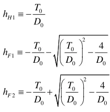
0 1
0
2 0 0 1
0 0 2 0 0 2
0 0
4
4
H
F
F
0
0
h
D
T T
h
D D D
T T
h
D D D
ion 1 Consider
e a sink in continuous time
0 then the steady state is a sink in dis- T
Proposit
(F
crete time if
> 0
h .
1) Let the steady state b
igure 1).
1.1) If T02 < 4D , < H1
h h and a source if hH1<h.
1.2) If T02 > 4D0,then the steady state is a sink if 0 <h
1
<hF , a saddle if F1<h<hF2and source if hF2<h
If the steady ddle in contin me,
h
state is a sa
. s ti
2) uou
then the steady state is a saddle in discrete time if
2
0 <h<hF and source if hF2<h (Figure 2).
3) If the steady state is a source in continuous time, th
generically undergoes a Hopf bifurcation at
en the source property is preserved whatever h> 0 (Figure 3).
The system
1
H
h and flip bifurcations at hFi, i= 1, 2.
Proof From (7) and (8), it is po ible toss plot a curve
1 h ,D h1
for each one of these different cases:
T
2 1 2 0
T T
1= 1 1
D T D0 given
T D0, 0
.state is a co
1) Assume that the steady ntinuous
tim
sink in
e: T0< 0 <D0. According to (8), D1>T11. Focus
on two T02 < 4D0 and (1.2 0.
1.1) If T02 < 4D0 ways 2
0 >
D h
cases: (1.1) ) T02 > 4
T h
2 D4
, then al 0 0,
that is T1 1 <D1.
hat is if
So, the steady
1< 1
D , t < 1
state is a sink if H
h h , and a source if h>hH1. This
rresponds pper parabola in 1.
In-creasing h away from zero means moving away from the point where h= 0, along the parabola.
case co to the u Figure
-2 2
2
-2 source
sink
case (1.2)
T D1
1
hH1
hF1 case (1.1)
saddle
h = 0
Figure 1. Sink in continuous time.
-2 2
-2 2
saddle source
T D1
1
hF2 T < 00 > 0
[image:3.595.360.486.360.740.2]h = 0
Figure 2. Saddle in continuous time.
-2 2
-2 2
source
T D1
1
h = 0
[image:3.595.114.227.560.675.2]1.2) If only if
2
2 0 > 4 0,
T D then D1< T1 1 if and 1< <
F
h h hF . In addition, D1< 1 if and only if
1
< H
h h . We notice also that 0 < F1<hH1<hF2. Then,
dy state is a sink if h 0 < <
the stea h hF1, a saddle if
1< < 2
F F
h h h and a source if is case
corre-lower parabola in 1.
2) Assume now that the steady state is a
2<
F h
Figure
h. Th sponds to the
saddle in con- tinuous time: D0< 0. According to (8), D1<T11. We
observe that hF1< 0 <hF2 and that D1> 1 and
only if hF1<h , the steady addle if
0 < <
1
T
if
ate is a s
2
F hus
<h . T st
2
F
h rce if hF2< .h If T0< 0 (T0> 0),
heh and a sou
the curve 0 is represented by t
on- tin
s cas
backward lo
ward. Simply observe that, in the case (3
2.2. Forward-Looking Discretizations
tization
1 (9)
of system (5) around the common steady state
T h D h1 , 1 :h>
ghtward) branch of para
leftward (ri bola in Figure 2.
3) Assume now that the steady state is a source in c uous time: T0 and D00. (7) and (8) imply T1> 2
and D1>T11 for every > 0 . Therefore the
property is preserved what h> 0. The branch of
parabola in Figure 3 represents thi e.
Corollary 2 (topological equivalence in h
ev
source er
oking) In any case of Proposition 1, there exists a nonempty interval
0,h for the discretization step h where the stability properties of the continuous-time sys- tem are preserved.Proof Straightfor ), h=.
We linearize now the forward-looking discre
xn1xnhf xn
= 0 f x to obtain
11 = 1 = 0
n n
dx J dx IhJ dxn
Differently from the previous case, the Jacobian
ma-trix of system (9)
0
1 1=
J IhJ is no longer linear in h. The trace and the determinant of J1 are now given
by
1= 2 0
T hT D1
2
1 2 1
0 0
1
= = 1
1
D T
hT h D
h D D0 1
As above, we set three critical values: hH2T D0 0 , 2
0 0 3
0 0 2 0 0 4
0 0
4
4
F
F
T T
h
D D D
T T
h
D D D
0
0
Proposition 3 Consider h> 0.
1) If the steady state is a sink in continuous time, then the sink property is preserved in discrete time whatever
. > 0 h
2) Let the steady state be a saddle in continuous time. 2.1) If D1> 0, then the steady state is a saddle.
< 0 D
2.2) If 1 , then the steady state is a saddle if
4
0 <h<hF and a sink if 4 .
3) Let the steady state be a source in continuous time. <
F
h h
3.1) Let D1< 0. If
20 0 < 4 0
T D D , then the source
property is preserved whatever h> 0. If
T D0 0
2> 4D0,then the steady state is a source if 0 <h<hF3 or
, and a saddle if
h hF3<h<hF4.
4<
F h
3.2) Let D1> 0. If
2 0 00 < <
0, then the steady
state is a source if 2
< 4
T D D
H
h h and a sink if 2 .
If
< H
h h
2 0 0 > 4T D D0, then the steady state is a source if
, a saddle if
3
F 3 4
<
h h hF <hhF and a sink if 4 .
The system generically undergoes a Hopf bifurcation at
< F
h h
2
H
h and flip bifurcations at Fi
Proof The proof is similar to that of Proposition 1. See Bosi and Ragot [4] for more details.
h , i= 3, 4.
Corollary 4 (topological equivalence in forward looking) In every case of Proposition 3, there exists a nonempty interval
0,h for the discretization step h where the stability properties of the continuous-time system are preserved.Proof Straightforward. Simply observe that, in cases (1) and (2.1), h=. The same happens in the case (3.1) if
T D0 0
2< 4 D0
n
.
2.3. Hybrid Discretizations
In economics, many higher-dimensional models require a hybrid discretization to recover the equivalence between discrete and continuous time, that is a mix of discretiza- tion in backward and forward looking. Without loss of generality, we consider a system where the first equation is discretized backward and the second one forward. Thus, the system of differential Equations (5) becomes:
1n 1 1n 1 1n, 2
x x hf x x (10)
2n 1 2n 2 1n 1, 2n 1
x x hf x x
(11)The steady state is invariant to the choice of time and to the type of discretization (backward/forward). The trace and the determinant of the Jacobian matrix J1 of
the hybrid system (10)-(11) become
0 0
1
2 2
= 2 1
h T hD T
h f x
(12)
2
0 0
1 1
2 2 2 2
= 1 = 1
1 1
hT h D
D T
h f x h f x
(13)
Notice that, in the particular case f2 x2= 0, (12)
and (13) write
2
1 1
1 0
= 1
= 1
T D h
D hT
0
Let
2
0 22 0 22
5
0 0
2 2 4
F
T f T f
h
D D
D0
2
0 22 0 22
6
0 0
2 2 4
F
T f T f
h
D D
D0
where f22 f2 x2.
Proposition 5 Consider h> 0.
1) Let 22 .
1.1) If the steady state is a sink in continuous time, then the steady state in discrete time is a sink if
0
f
6
0 <h<hF , and a saddle if 6 .
1.2) Let the steady state be a saddle in continuous time.
<
F
h h
1.2.1) If
T02f22
D024 D0<0 or T0> 2f22,then the steady state is a saddle point.
1.2.2) If
T02f22
D024 D0>0 T0< 2f22 5<
and ,
then the steady state is a saddle if 0 <h hF or
, and a source if
6< 5 6
F
h h hF <h<hF .
1.3) If the steady state is a source in continuous time, then the steady state is a source if 0 <h<hF6 and a
saddle if hF6<h.
> 0
f
2) Let 22 with 22. All the previous cases
hold, provided we restrict the analysis to the interval
< 1
h f
0,1 f22
.The system generically undergoes a Hopf bifurcation at hH2 and a flip bifurcation at Fi
Proof The proof is similar to that of Proposition 1. See Bosi and Ragot [4] for more details.
h , i= 5, 6.
Corollary 6 (topological equivalence in hybrid look- ing). In every case of Proposition 5, there exists a non-
empty interval for the discretization step h where
the stability properties of the continuous-time system are preserved.
0,h
Proof Straightforward. Simply observe that, in the case (1.2.1), h=.
3. Ramsey Model
In the seminal Ramsey [1], the planner maximizes the
undiscounted dynastic utility:
, un-0 u ct u c dt
t t t t
k k c f k
der a resource constraint where t
and t denote the individual capital and consumption.
The initial endowment is given.
k
k c
0
The intensive production function f k is strictly increasing and strictly concave in the capital intensity and satisfies the Inada conditions. The felicity u c
is also strictly increasing and strictly concave in the con- sumption level. c denotes the bliss point, that is the steady state value of consumption: c= f
k kwith f'
k = .The planner maximizes the Hamiltonian:
t t t t t
to find the first-order conditions:
=
t t t
k f k k c t
(14)
= '
t t f kt
(15)
where ct =c
t u' 1
t H u c u c f k k c
t
t
c
t
. The strict concavity of u ensures that is a well-defined function of the multi- plier .
In discrete time, the planner maximizes
=0 t
t u c u c
1
t t t k k
under a sequence of resource con-
straints: , to obtain the first-
order conditions:
t k c f kt
1 =
t t t t t
k k f k k c
(16)
1= 1 1
'
t t f kt
(17)
We want to prove that the discrete-time system (16)- (17) is a discretization of the continuous-time system (14)- (15).
Proposition 7 The discrete-time Ramsey model comes from a first-order hybrid Euler discretization of the con- tinuous-time model, that is a backward-looking discreti- zation of the resource constraint (14) and a forward- looking discretization of the Euler Equation (15), with a unit step.
Proof Under the backward-looking linear discretiza- tion of the continuous-time resource constraint (14):
t h t t t t
k k h f k k c (18)
we recover exactly the discrete-time resource constraint (16) with a unit discretization step ( ). However, the intertemporal arbitrage requires a forward-looking dis- cretization. Focus on (15) and apply (4):
= 1 h
= '
t h t h t h f kt h
to obtain
1 '
t t h h f kt h
(19)
which gives exactly the discrete-time Euler Equation (17) under a unit discretization step h= 1.
The forward-looking discretization of (15) is more suitable to capture saving decisions. Indeed, the expected productivity affects the arbitrage between consumption today and consumption tomorrow.
Let us consider the steady state. For all the three dy- namical systems (14)-(15), (16)-(17) and (18)-(19) the steady state is defined by: '
=f k and
= =
c c f k k (assumptions on technology and
preferences ensure its existence and uniqueness).
Focus now on the stability properties. The Jacobian matrix J0 of the continuous time system (14)-(15) is
given by:
0
0 =
0 Ak J
B k
where A
1
> 0, B
1
>0 with
> 0' ''
u c u c c
, kf'
k f k 0,1
=
1
< 0'' '
kf nd the
and k f k . The trace a
determinant in continuous time are and
0.
le-path y
prop-erty.
The hybrid Euler discretization ( 9) is consistent
position 8 The steady state of the discretized m
h.
0= 0
T
0= <
D AB
Notice that D0< 0 implies the sadd stabilit
18)-(1 with the continuous-time case.
Pro
odel is a saddle point (as in the continuous-time case) whatever the discretization step
Proof The Jacobian matrix J1 of the hybrid Euler
discretization (18)-(19) is:
1 2
1 =
1 h J
hB k Bh
Ak A
where A and B are defined above. The trace and deter-
minant become B and . We obt
1 r th ath stability
r the discreti h
room for bifur
s- cr
REFERENCES
[1] F. Ramsey, “ of Saving,”
Eco-nomic Journal , pp. 543-559.
2
1= 2
T h A
and we recove
1= 1
D e saddle-p
ain
1 1
property, whateve zation step . There is no
cations, as in the continuous-time case. Therefore, the saddle-path stability is a robust property of the Ramsey model because it holds whatever the di
1D <T
etization step.
A Mathematical Theory , Vol. 38, No. 152, 1928
doi:10.2307/2224098
[2] H. Krivine, A. Lesne and J. Treiner, “Discrete-Time a Continuous-Time Mod
nd elling: Some Bridges and Gaps,”
Mathematical Structures in Computer Science, Vol. 17, No. 2, 2007, pp. 261-276.
doi:10.1017/S0960129507005981
[3] P. A. Samuelson, “The Stabil
parative Statics and Dynamics,” Econometrica
ity of Equilibrium: Com-, Vol. 9Com-, No. 2, 1941, pp. 97-120. doi:10.2307/1906872