Easy Simplex (AHA Simplex) Algorithm

(1)

ISSN Online: 2327-4379 ISSN Print: 2327-4352

DOI: 10.4236/jamp.2019.71003 Jan. 10, 2019 23 Journal of Applied Mathematics and Physics

Easy Simplex (AHA Simplex) Algorithm

A. H. Ansari

Kejriwal Institute of Management and Development Studies, Ranchi, India

Abstract

The purpose of this research paper is to introduce Easy Simplex Algorithm which is developed by author. The simplex algorithm first presented by G. B. Dantzing, is generally used for solving a Linear programming problem (LPP). One of the important steps of the simplex algorithm is to convert all unequal constraints into equal form by adding slack variables then proceeds to basic solution. Our new algorithm i) solves the LPP without equalize the con-straints and ii) leads to optimal solution definitely in lesser time. The goal of suggested algorithm is to improve the simplex algorithm so that the time of solving an LPP will be definitely lesser than the simplex algorithm. According to this Easy Simplex (AHA Simplex) Algorithm the use of Big M method is not required.

Keywords

Linear Programming, Simplex Algorithm, Optimal Solution, Easy Simplex Algorithm, AHA Simplex Algorithm

1. Introduction

One of the most dynamic areas of applied mathematics is linear programming (LP). The simplex method was first time implemented by George Barnard Dant-zig during Second World War, then the method was introduced by [1], the simplex algorithm is an iterative procedure for solving linear programming problem in finite number of steps. It provides an algorithm which consists of moving from one vertex of feasible region to another vertex of feasible region in such a manner that the value of objective function at the neighboring vertex is near to optimal than at the previous vertex. The procedure is repeated until the optimal solution reached and since the number of vertices are finite, therefore the method leads to an optimal vertex (Optimal solution) in a finite number of repetition of process or indicate about the existence of unbounded or infeasible

How to cite this paper: Ansari, A.H. (2019) Easy Simplex (AHA Simplex) Algo-rithm. Journal of Applied Mathematics and Physics, 7, 23-30.

https://doi.org/10.4236/jamp.2019.71003

Received: December 3, 2018 Accepted: January 7, 2019 Published: January 10, 2019

Copyright © 2019 by author(s) and Scientific Research Publishing Inc. This work is licensed under the Creative Commons Attribution-NonCommercial International License (CC BY-NC 4.0). http://creativecommons.org/licenses/by-nc/4.0/

(2)

DOI: 10.4236/jamp.2019.71003 24 Journal of Applied Mathematics and Physics

solution. This method tests adjacent vertices of the feasible set (which is a poly-tope) in succesion so that each new vertex improves the objective function value or leaves it unchanged. The Simplex method is very efficient in practice. How-ever, in [2], Klee and Minty gave an example of a linear programming problem in which the polytope is a distortion of an n-dimensional cube. They show the number of arithmetic operations in the simplex algorithm grows exponentially with the number of variables. In [3], Khachiyan proposed the first polynomial algorithm, the ellipsoid method. In [4], Karmarkar suggested the second poly-nomial-time algorithm, which appears to be more efficient than Simplex method, especially when the problem size increases above some thousands of variables

[5]. These authors motivate me to think in different procedure by which the time of solving an LPP should take less time with the less number of variables. One of the important steps of the simplex algorithm is of course selection of ba-sis-entering variable. Dantzig simplex method still seems to be the most efficient procedure for majority of practical problems, especially for small problems.

In this research paper, I proposed an easy simplex algorithm and defined it as AHA simplex algorithm (by the short name of author). The algorithm will defi-nitely take less time in solving an LPP with the help of assumption that there is no basic variables at initial stage, the objective function value is zero at this stage with all non basic variables which is same as the simplex method. The idea is to improve the objective function value in each iteration by entering non basic va-riable in blank set of basic vava-riables. Then, we do the calculation according to the easy simplex algorithm which is explained in the coming sections with illu-stration.

2. Notation

The general form of an LPP is

1 1 2 2

Max z c x c x= + + + c xn n

11 1 12 2 1 1

21 1 22 2 2 2

1 1 2 2

Subject to ,

,

n n

m m mn n m

a x a x a x b

+ + + ≤

LPP (2.1)

Non negative condition x x1, , ,2 xn ≥0

It can be written in Matrix form as:

T

Max

z c X

=

Subject to

0

AX b X

≤

≥ LPP (2.2)

where

1 Column Vector

X n= × _,

Coefficient Matrix

A m n= × _,

1 Column Vector

(3)

1 Row Vector

c= ×n

If the above problem has only two vectors, then it can solve easily by Graphi-cal method. If the LPP has more than two variables, then simplex method is ap-propriate and powerful method to solve these types of problems.

3. Proposed AHA Simplex Simulation Algorithm

3.1. The Simplex Algorithm

To solve any LPP using simplex algorithm, the existence of an initial basic feasi-ble solution is always assumed. Consider the LPP (2.2). The steps for the com-putation of an optimum solution are as follows:

Step 1. Check whether the objective function of the given LPP is to be max-imized or minmax-imized. If it is to be minmax-imized then we convert it into a problem of maximizing it by using the result Maximum z = −Minimum (−z)

Step 2. Check whether all

b i

i

(

=

1,2,3, ,

m

)

are non negative. If any one of

i

b is negative then multiply the corresponding inequation by −1, so as to get all

(

1,2,3, ,

)

i

b i

=

m

must be non negative.

Step 3. Convert all the inequations of the constraints into equations by intro-ducing slack and/or surplus variables in the constraints. Put the costs of these variables equal to zero.

Step 4. Obtain an initial basic feasible solution to the problem in the form 1

B

x

₌

B b

− _{and put it in the first column of the simplex tableu.}

Step 5. Compute the net evaluations

z c j

_j

−

_j

(

=

1,2, ,

n

)

using the relation

j j B j j

z c− =C y C− where 1

j j

y ₌B a− _{examine the sign}

j j

z c−

a) If all

(

zj−cj

)

≥0 then the initial basic feasible solution is an optimal

ba-sic feasible solution.

b) If at least one z cj− j<0, proceed to the next step.

Step 6. If there is more than one z cj− j<0 then choose the most negative

of them. Let it be for j r=

a) If all

y

ir

≤

0 (

i

=

1,2,3, ,

m

)

then the problem is an unbounded solution

to the given problem.

b) If at least one

y

ir

>

0 (

i

=

1,2,3, ,

m

)

then corresponding vector yr is

known as pivotal column, enter the basis yB.

Step 7. Compute the ratios Bi; 0 ir ir

x _y

y

 

∀ >

 

  and choose the minimum ratio.

Suppose the vector yk have the minimum ratio then it is known as pivotal row,

will leave the basis yB. The common element of pivotal column and pivotal row

is pivotal element ykr.

Step 8. Convert the pivotal element to unity by dividing its row by pivotal element ykr and all other elements in pivotal column to zero by making use of

the relations:

(

)

kj

(

₍

)

₎

; 1,2,3, , , ij

kr

y Old

y New j n i k

y Old

(4)

(

)

(

)

kj

(

)

₍

ir

₎

(

)

; 1,2,3, , , , 1,2,3 , ,

ij ij

kr

y Old y Old

y New y Old i m i k j n

y Old

×

= − ∀ = ≠ =

Step 9. Go to step 5 and repeat the computational procedure until either an optimum solution is obtained or there is an unbounded solution.

3.2. The Easy Simplex (AHA Simplex) Algorithm

Consider the same LPP (2.2). Without loss of generality the objective function can be written as objective inequation:

1 1 2 2

Max z c x c x≤ + + + c xn n (3.2.1)

or

T

Max 1 c z 0

x

 

 − _{ }≤

 _{  } (3.2.2)

[

]

Subject to 0 A z b

x

  ≤  

 

(3.3.3)

0

X ≥

_(3.3.4)

Steps for the computation of an optimum solution are as follows:

Step 1. Check whether the objective function of the given LPP is to be max-imized or minmax-imized. If it is to be minmax-imized then we convert it into a problem of maximizing it by using the result Maximum z = −Minimum (−z).

Step 2. Check whether all

b i

i

(

=

1,2,3, ,

m

)

are non negative. If any one of

i

b is negative then multiply the corresponding inequation by −1, so as to get all

(

1,2,3, ,

)

i

b i

=

m

must be non negative.

Step 3. Examine the sign of all decision variables in objective inequation −cj

a) If all − ≥cj 0 then the solution is an optimal solution where z=0 and

(

)

0 1,2, ,

j

x

= ∀ =

j

n

.

b) If at least one − <cj 0, proceed to the next step.

Step 4. If there is more than one − <cj 0 then choose the most negative of

them. Let it be for j r=

a) If all

a

_ir

≤

0 (

i

=

1,2,3, ,

m

)

then the problem is an unbounded solution to the given problem.

b) If at least one

a

_ir

>

0 (

i

=

1,2,3, ,

m

)

then corresponding vector xr is

known as pivotal column, enter into the basis yB.

Step 5. Compute the ratios i ; 0, 1,2,3, , ir

ir

b _a _i _m

a

 

∀ > =

 

  and choose the

minimum ratio. Suppose k ; 0 kr kr

b _a

a

 

∀ >

 

  have the minimum ratio then it is

known as pivotal row, which is initially blank will fill by entering the variable

r

x into the basis yB. The common element of pivotal column and pivotal row

is pivotal element akr.

Step 6. Convert the pivotal element to unity by dividing the row by pivotal element

(

)

kj

(

₍

)

₎

kr

a Old a New

a Old

(5)

by making use of the relations:

(

)

(

)

{

(

)

}

(

)

;

j j r kj j

c New c Old c Old a New c

− = − − − × ∀

(

)

(

)

{

(

)

}

(

)

; ,

ij ij ir kj ij

a New =a Old − a Old ×a New ∀a i k≠

Step 7. Go to step 3 and repeat the computational procedure until either an optimum solution is obtained or there is an unbounded solution.

4. Numerical Illustrations

Illustration 1: Solve the following LPP.

1 2 3 4

Max z=12x +20x +18x +40x

1 2 3 4

Subject to 4 9 7 4 6000,

3 40 4000,

and , , , 0

x x x x

x x x x

x x x x

+ + + ≤

≥

Solution: Since there is Maximization type objective function and all con-straints are less than type. Then we use the AHA Simplex method as

1 2 3 4

Max z−12x −20x −18x −40x ≤0

1 2 3 4

Subject to 4 9 7 4 6000,

3 40 4000,

and , , , 0

x x x x

x x x x

x x x x

+ + + ≤

≥

Initial Table (Table 1)

Basic Variables x1 x2 x3 x4 bi

−12 −20 −18 −40 ≤ 0

4 9 7 10 ≤ 6000

1 1 3 40 ≤ 4000

The most negative coefficients of x4 in objective inequation is – 40 in

(

Row

0

)

in Table 1, so the entering variable is x4. Minimum positive ratio is 100, so the x4 enter into

(

Row

2

)

. Therefore pivotal element is 40.

(

)

( )

2 2

40 R New

=

R Old

÷

(

)

(

)

(

)

0 0 40 2

R New =R Old + ×R New

(

)

(

) (

)

(

)

1 1 10 2

R New =R Old + − ×R New

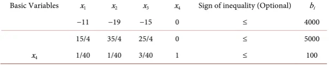
First Iteration (Table 2)

Basic Variables x1 x2 x3 x4 Sign of inequality (Optional) bi

−11 −19 −15 0 ≤ 4000

15/4 35/4 25/4 0 ≤ 5000

x4 1/40 1/40 3/40 1 ≤ 100

[image:5.595.206.541.633.700.2]

(6)

(

Row

0

)

in Table 2, so the entering variable is x2. Minimum positive ratio is

5000 571.429

35 4 ≈ , so the x2 enter into

(

Row

1

)

. Therefore pivotal element is 35/4.

(

)

( )

1 1

35 4

R New

=

R Old

÷

(

)

( )

(

)

0 0

19

1

R New

=

R Old

+ ×

R New

(

)

(

)

{

(

)

}

(

)

2 2 1 40 1

Second Iteration (Table 3)

−20/7 0 −10/7 0 104,000/7

x2 3/7 1 5/7 0 4000/7

x4 1/70 0 2/35 1 600/7

The most negative coefficients of x1 in objective inequation is −20/7 in

(

Row

0

)

in Table 3, so the entering variable is x1. Minimum positive ratio is

4000 7 1333.33

3 7 ≈ , so the x1 enter into

(

Row

1

)

(

)

( )

1 1

3 7

R New

=

R Old

÷

(

)

(

) (

)

(

)

0 0

20 7

1

R New

=

R Old

+

×

R New

(

)

(

)

{

(

)

}

(

)

2 2 1 70 1

Third Iteration (Table 4)

0 20/3 10/3 0 56,000/3

x1 1 7/3 5/3 0 4000/3

x4 0 −1/30 1/30 1 200/3

Since the all coefficients of xj in objective inequation in

(

Row

0

)

of Table 4 is either zero or positive, means the optimal solution achieved, and optimal solu-tion always lies at extreme point thus the optimal solusolu-tion is as 56000

3

z= _,

1 4000₃

x = _, ₄ 200

3

x =

Illustration 2: Solve the following LPP.

1 2

Max z=4x +3x

1 2

Subject to 50,

2 80,

3 2 40

and , 0

x x

x x

x x

+ ≤

+ ≥

(7)

Solution: Since there is Maximization type objective function and some con-straints are in greater than form, so subtract extra variables as follows.

1 2 3 4

Max z=4x +3x +0x +0x

1 2

1 2 3

1 2 4

1 2 3 4

Subject to 50,

2 80,

3 2 40

and , , , 0

x x

x x x

x x x x

+ ≤

+ − ≤

≥

Then we use the AHA Simplex method as

Initial Table (Table 5)

Basic Variables x1 x2 x3 x4 Sign of inequality (Optional) bi

−4 −3 0 0 ≤ 0

1 1 0 0 ≤ 50

1 2 −1 0 ≤ 80

3 2 0 −1 ≤ 40

The most negative coefficients of x1 in objective inequation is—4 in

(

Row

0

)

of Table 5, so the entering variable is x1. Minimum positive ratio is 40/3, so the

1

x enter into

(

Row

3

)

. Therefore pivotal element is 3.

(

)

(

)

3 3 3

R New =R Old ÷

(

)

( )

(

)

0 0

4

3

R New

=

R Old

+ ×

R New

(

)

( ) ( )

(

)

1 1

1

3

R New

=

R Old

+ − ×

R New

(

)

( ) ( )

(

)

2 2

1

3

R New

=

R Old

+ − ×

R New

First Iteration (Table 6)

0 −1/3 0 −4/3 160/3

0 1/3 0 1/3 110/3

0 4/3 −1 1/3 200/3

x1 1 2/3 0 −1/3 40/30

The most negative coefficients of x4 in objective inequation is −4/3 in

(

Row

0

)

of Table 6, so the entering variable is x4. Minimum positive ratio is

110 3 110

1 3 = , so the x4 enter into

(

Row

1

)

(

)

(

)

1 1 1 3

R New =R Old ÷

(

)

(

) ( )

(

)

0 0 4 3 1

R New =R Old + ×R New

(

)

(

)

{

( )

}

(

)

2 2 1 3 1

(

)

( ) ( )

(

)

3 3

1 3

1

(8)

Second Iteration (Table 7)

0 1 0 0 200

x4 0 1 0 1 110

0 1 −1 0 30

x1 1 1 0 0 50

Since the all coefficients of xj in objective inequation

(

Row

0

)

of Table 7 is either zero or positive, means the optimal solution achieved, and optimal solu-tion always lies at extreme point thus the optimal solusolu-tion is as z=200_,

1 50

x = _, x₄=110_.

5. Conclusion

Since the Simplex Algorithm is an algorithm to solve the Linear Programming Problem (LPP) for more than two variables (also applicable in two variable) in such a manner that the optimal solution is achieved after a fixed number of ite-ration, the proposed Easy (AHA) Simplex Algorithm is a better algorithm to solve an LPP, because it has lesser calculation because the number of variables are less and steps (in some cases) and take lesser time than the Simplex algo-rithm.

Conflicts of Interest

The author declares no conflicts of interest regarding the publication of this pa-per.

References

[1] Dantzig, G.B. (1951) Linear Programming. Applied Mathematics Series 15, National Beuro of Standards, 18-21.

[2] Klee, V. and Minty, G.J. (1972) How Good Is the Symplex Algorithm? In: Shisha, O., Ed., Inequalities, III, Academic Press, New York, 159-175.

[3] Khachiyan, L.G. (1979) A Polynomial Algorithm in Linear Programming. Soviet Mathematics Doklady, 20, 191-194.

[4] Kramaker, N. (1984) A New Polynomial-Time Algorithm for Linear Programming.

Combinatorica, 4, 373-395. https://doi.org/10.1007/BF02579150