Munich Personal RePEc Archive
Exchange Rate Induced Export Quality
Upgrading: A Firm-Level Perspective
Hu, Cui and Parsley, David and Tan, Yong
31 July 2017
Online at
https://mpra.ub.uni-muenchen.de/80506/
Exchange Rate Induced Export Quality
Upgrading: A Firm-Level Perspective
†Cui Hua David Parsleyb Yong Tanc‡
a: School of International Trade and Economics, Central University of Finance
and Economics
b: Owen Graduate School of Management, Vanderbilt University
c: Department of Economics, Vanderbilt University
Abstract
This paper explores the impact of exchange rate fluctuations on exported product quality. Existing studies of quality upgrading stress the link between home country depreciation and increased access to export markets. Our focus in this study is on the complimentary effect of an import currency appreciation (i.e., the domestic currency appreciates relative to the sourcing country’s currency). Our main finding is that firms upgrade their export quality in response to an import currency appreciation. We first develop a partial equilibrium model to reveal the mechanism: an import currency appreciation that makes imported intermediates cheaper allows firms to switch to higher quality intermediates, which in turn, increase export quality. Using Chinese Customs data during 2000-2006, we find that an import appreciation increases both import, and export quality. Furthermore, export quality increases more for less productive firms, and for firms exporting to developed countries.
Keywords: Import Appreciation · Quality Upgrade · Import Quality· Export Quality JEL Classification: F10·F12·F13
†Contact information: [email protected](C. Hu),[email protected]
(D. Parsley). yongtan [email protected](Y. Tan)
1. Introduction
It is widely believed that exchange rate fluctuations are crucial to firms’ export
performance. A considerable number of papers document the impact of exchange
rate fluctuations on export prices and volumes (Cushman, 1983; Dell, 1999; Mc
Kenzie, 1999; Forbes, 2002; Marquez and Schindler, 2007; Cheung et al., 2009;
Thorbecke and Simith, 2010; Berman et al., 2012; Li et al., 2015; Chen and
Ju-venal, 2016). However, the specific mechanism that exchange rate fluctuations
affect export quality is less well understood. One avenue suggested by recent
the-oretic work emphasizes the role that input quality plays in final product quality
(Kugler and Verhoogen, 2012; Hallak and Sivadasan, 2013). Presumably, higher
quality intermediate inputs are more costly. In this paper, we argue that firms
may upgrade their export quality by capitalizing on exogenous import currency
appreciation (the domestic currency appreciates relative to the currency in the
sourcing countries).
One of the most salient features of international trade is that a large portion
of exporters are simultaneous importers (e.g. Amiti et al., 2014). This suggests
that exchange rate movements affect the price of imported intermediate inputs,
which in turn, affect these firms’ choice of imported intermediate input quality.
This paper attempts to provide empirical evidence on the link between import
exchange rate fluctuations and the quality of traded products.
In order to uncover the links between exchange rate movements and traded
product quality, and to guide our empirical strategy, we develop a theoretic
frame-work to study heterogeneous firm-level quality responses to import exchange rate
that firms use domestic and foreign imported intermediates to produce final
prod-ucts. Import prices are influenced by both the quality of imported intermediates
and the import exchange rate. To produce high quality products (for domestic
or foreign markets), firms are required to use both high quality domestic and
im-ported intermediate inputs. In equilibrium, more productive firms tend to import
higher quality intermediates and export higher quality products. In response to
an import exchange rate appreciation, firms switch to (previously) more
expen-sive and higher quality intermediates, which in turn, improves the quality of their
exported products.1 The model further predicts that if the quality transferring
between intermediate inputs and final products exhibits diminishing returns, more
productive firms will upgrade their product quality less when facing an import
appreciation. This is because it is more costly to upgrade the product quality if it
is already high, and as such, both import and export quality of more productive
(higher quality) firms reacts less to import appreciations.
We test the predictions of the model with a rich dataset of Chinese trading
firms during 2000-2006 period. A distinctive feature of these data is that they
provide firm-level imports by source countries and exports by destination country,
at HS8-digit product codes. Having import information allows us to construct
a firm-level effective import exchange rate, its import sophistication, and import
intermediates quality. Information on exports provides us with a measure of
ex-port product quality. Our empirical results, on the one hand, indicate that a 10%
import currency appreciation increases firm-level export quality by 0.8%, and this
1
quality increase is mainly driven by firms that engaged in ordinary trade.2 On
the other hand, our results demonstrate that a 10% import currency appreciation
tends to increase firm-level import sophistication and quality by 0.7% and 1.5%,
respectively. Furthermore, we find that the import price in developed countries
fall is twice that in developing countries in response to an import currency
appre-ciation. Without quality upgrading, this result contradicts the findings in Chen
and Juvenal (2016) and Bernini and Tomasi (2015), who find that exchange rate
pass-through is decreasing in traded product quality.3
This paper is closely related to the recent, growing literature on the connections
between exchange rate fluctuations and firm-level export performance, especially
studies on exchange rate pass-through (Atkson and Burstein, 2008; Amiti et al.,
2014; Berman et al., 2012; Bergsten, 2010; Chatterjee et al., 2013; Campa and
Goldberg, 2005; Gopinath and Rigobon, 2008; Knetter, 1993; Giri, 2012;
Berni-ni and Tomasi, 2015), and to the literature tracing imported inputs and export
performance. Broadly, the exchange rate pass-through (ERPT) literature has
fo-cused on three channels leading to incomplete pass-through. The first channel
at-tributes incomplete pass-through to import and export price rigidities (Gopinath
and Rigobon, 2008), i.e., an incompletely adjusted local price results in a low level
of exchange rate pass-through. The second channel is pricing-to-market (Atkson
and Burstein,2008;Amiti et al.,2014), in which exporting firms endogenously
ab-sorb exchange rate fluctuations by adjusting their markups, which stabilizes trade
price fluctuations. Third, a large literature explains incomplete pass-through by
2
Both export and import quality are estimated followingKhandelwal et al.(2013).
3
introducing local distribution costs (Berman et al.,2012;Li et al.,2015; Chen and
Juvenal, 2016; Campa and Goldberg, 2005; Chatterjee et al., 2013; Giri, 2012).
Since distribution costs, which may be a large share of the price, are paid in
lo-cal currency, the impact of exchange rate fluctuations on import prices will be
mitigated.
Second, our work relates to the literature studying the interaction of importing
materials and exporting performance. Kasahara and Rodrigue(2008), for instance,
document that using imported intermediates effectively improves the
productiv-ity of Chilean manufacturing firms. Chevassus-Lozza (2013), Feng et al. (2016)
and Bas and Strauss-Kahn (2015) separately find that input trade liberalization
boosts both the downstream industries and firms’ exports, as well as increasing
the quality of export products. Our work is similar in spirit toBernini and Tomasi
(2015), who relate firm-level ERPT to the quality of imported intermediate inputs.
We endogenize the intermediate input quality choice resulting from exchange rate
movements, and trace the downstream effects on export quality.
Importantly, our work contributes to this exchange rate incomplete pass-through
literature by introducing a firm-level endogenous quality adjustment. Faced with
an import currency appreciation, a representative firm imports higher quality, and
hence (formerly) more expensive intermediates, which lowers import price
pass-through. As a consequence, the firm produces higher quality export products,
and it charges a higher markup (price) in export destinations. This shows up as
increased pass-though to export destinations.
Empirically, we focus on China primarily due to our extensive data set on
firm-level imports and exports by country - which permits an examination of our
presents a promising focal point due to its emerging status and its rapid trade
growth. Moreover, recent studies, e.g., Pula and Santababara (2011) emphasize
the prevalence of quality upgrading by Chinese firms. Third, other studies, e.g.,
Li et al. (2015) focus on China’s high export pass-through.4
The rest of this paper proceeds as follows. Section 2 outlines the economic
model. Section 3 describes the dataset and the construction of the variables that
will be used in our tests. The results are presented and discussed in section 4.
Section 5 concludes.
2. Model
In this section, we develop a theoretical framework linking a firm’s import and
export quality choices to import exchange rate changes. We use this framework
to formulate testable implications.
In order to focus our analysis on the relationship of import exchange rate
changes and firm-level import and export quality, we make a number of
assump-tions. First, similar to Amiti et al. (2014), we do not model firms’ entry, exit, or
selection into exporting and importing, as we condition our analysis on the
sub-set of firms, which simultaneously import and export, and focus on their import
and export quality.5 Second, this model is partial equilibrium, hence we abstract
from the impact of import exchange rate changes on wages in each country, and
4
Li et al.(2015) estimate export Chinese pass-through at 96% - well above most other coun-tries: e.g., 79% for Belgian exporters (Amiti et al.,2014); 77% for Brazilian exporters (Chatterjee et al.,2013). Only two countries exhibit export pass-through similar to that of Chinese exporters, at nearly 100% for U.S. exporters (Knetter, 1993), and 92% for French exporters, (Berman et al.,2012)
5
aggregate demand in the export destinations; instead, we focus on the impact of
import exchange rate changes on firm-level import and export behaviors, i.e. the
wage and residual demand in each country are taken as exogenously given.6
2.1. Demand
We assume there are three countries in the world. The home country,C(China
in our case), a foreign country,F1 importing final products from the home country,
and another foreign country,F2 producing and exporting intermediate inputs and
exports. A representative export firm in the home country uses intermediate inputs
produced in country C and imported from country F2 to produce final products,
which will be sold in the home countryC and foreign countryF1. A representative
consumer’s preference in country C and F1 takes the following CES form:
U =
"Z
ω∈Ωj
[q(ω)x(ω)]σ−σ1
# σ σ−1
(1)
where q(ω) and x(ω) denote the quality and quantity of variety ω, respectively.
Representative firms can produce a variety with different quality for different
markets: qC for the home market, and qF1 for the foreign market. Exporters face
three types of costs for exporting: an iceberg trade cost τj, τj >1 if j =F1, and
τj = 1 if j = C; a fixed cost fj, and a per unit distribution cost in country j,
ηj =ηwj. Note that the distribution cost is paid in the local currency. wj is the
wage level in countryj and η is the amount of labor required for distribution. We
now discuss the firms’ export behavior in foreign country F1; the results can be
6
easily applied to the home country.
If an exporter from country C charges a price pF1 in the home currency for
its product exported to country F1, the price faced by consumers in the foreign
country is
pc
F1(ϕ) =
pF1(ϕ)τF1
eF1
+ηF (2)
where eF1 is the nominal exchange rate between the home country C and
for-eign country F1. ϕ is the productivity of the firm. An increase in eF1 implies a
depreciation of the domestic currency. The quantity demanded in F1 is
xF1(ϕ) =YF1P
σ−1
F1
pF1(ϕ)τF1
qF1(ϕ)eF1
+ηF −σ
(3)
where YF1, and PF1 denote the aggregate income and price index in country F1,
respectively. It is easy to see from equation (3) that for a given F.O.B price pF1,
a decrease in eF1 (foreign currency depreciation) will lead to a higher demand in
countryF1. Export profit in country F1 is:
πF1 =YF1P
σ−1
F1
pF1(ϕ)τF1
qF1(ϕ)eF1
+ηF −σ
[pF1(ϕ)−c(ϕ, eF2)] (4)
where c(ϕ, eF2) denote the unit production cost of the export product, which
de-pends on firm-level productivity and the exchange rate between the home country
2.2. Production
We build on Amiti et al. (2014) and Rodrigue and Tan (2016) to model the
cost structure of the representative firm and its import (export) quality choice.7
Consider a representative firm with productivity ϕ with the following production
function:
Y =ϕX (5)
where, X is the intermediate input. The production function (5) implies that
intermediates are the only input in the production, and the production function
features constant return to scale.
Intermediate input X consists of a bundle of intermediate goods indexed by
j ∈[0,1] and aggregated according to a Cobb-Douglas technology:
X =exp
Z 1
0
logXjdj
(6)
where each intermediate goodj can be made by combining two varieties purchased
from domestic country C and sourcing country F2:
Xj =
Z
ζ ζ+1
j +a
1
ζ+1
j M
ζ ζ+1
j
1+ζ ζ
(7)
where Zj and Mj denote the quantities of domestic and imported varieties of the
intermediate good j used in production, respectively. ζ+ 1 measures the
elastic-7
ity of substitution between domestic and imported varieties, and ζ + 1 > 1. aj
captures the relative importance of foreign variety, Mj, in producing intermediate
goodsXj. aj >1 (aj <1 ) indicates that the foreign imported variety,Mj, is more
(less) important in production relative to the domestic variety, Zj. Note that the
production of intermediate goodsXj is possible by using only the domestic variety
Zj. Imported variety Mj makes the production of Xj more efficient through the
relative importance parameter aj, and the ‘love-of-variety’ feature of the
produc-tion funcproduc-tion (7). To import foreign varieties, each firm needs to pay a fixed cost
f in terms of labor.
Each intermediate variety has been made using labor. Wages in the domestic
countryC and sourcing countryF2 are exogenously given by W and 1,
respective-ly.8 FollowingKugler and Verhoogen (2012), we assume the intermediate varieties
market to be competitive in both the domestic country C and the sourcing
coun-try F2. As such, Producers of intermediate varieties, Zj and Mj, earn zero profit.
Each intermediate variety differs in quality. The higher the quality, the more
la-bor required in production. Without loss of generosity, we assume that in both
the domestic and the sourcing countries, to produce any intermediate variety with
quality qj, the labor requirement is qj. Following Rodrigue and Tan (2016), we
assume that the quality of intermediate goodsXj depends on the minimum quality
of the domestic and imported intermediate varieties, and the quality of
interme-diate input X depends on the lowest quality of {Xj}j∈[0,1]. Finally, the quality of
8
intermediate input X affects the quality of products exported to country F1.
qXj = min{qZj, qMj}
qX = min{qXj}j∈[0,1]
qF1 =ϕq
α
X (8)
where qZj, qMj, qXj, qX, and qF1 denote the quality of Zj, Mj, Xj, X and products
exported to destination F1, respectively. α captures the concavity of the quality
cost curve: a higherαimplies a lower cost of increasing quality by a given amount.
We refer toαas the “quality transfer rate” in subsequent discussions. Equation (8)
indicates that productivity and quality are complementary,9 higher productivity
firms can produce higher quality final products using the same intermediate as a
low productive firm. Moreover, ifα <1, it would be harder to increase the quality
of final products by increasing the quality of intermediates. The quality function
structure implies that in equilibrium, a firm will choose intermediates such that
qXj =qXk for ∀j 6=k and qZj =qMj for∀j.
Equation (8) also implies that a firm needs to use intermediates with quality
q ϕ
1
α
in order to produce products with quality q. If a firm uses both domestic
and foreign intermediates to produce exported products with quality q, the prices
of domestic and foreign intermediates are Wϕq
1
α
and ϕq
1
α
eF2τF2. The total
production cost is R01Wϕq
1
α
Zjdj + R1 0 q ϕ 1 α
eF2τF2Mjdj +W f, where the last
term is the fixed import cost.10 Similar toAmiti et al.(2014), firm-level marginal
9
None of our results rely on the complementarity between the productivity and the interme-diate quality. For instance, all our results continue to hold if we assumeqF1 =q
α X .
10
production cost with qualityq is
c(ϕ, eF2, q) =ϕ
−1+ααW q
1
α
B (9)
B = exp Z 1
0
logbjdj
bj =
1 +aj eF
2τF2
W
−ζ1ζ
whereτF2 is the iceberg trade cost between the home country and foreign country
F2. Equation (9) implies that an appreciation in the home currency (a decrease in
eF2) leads to a decline in the price for importing (in home currency) intermediates.
Notice that the cost function defined in equation (9) is for firms with positive
imports. We do not analyze the firm-level import decision here, but we argue
that only firms with sufficiently high productivity choose to pay the fixed import
cost, f, given the cost structure in (9). If a firm is not engaged in importing, its
marginal production cost (with qualityq) is given by: c(ϕ, q) = ϕ−1+ααW qα1.11 The profit function (4) and cost function (9) together give the optimal export
price:
pF1(ϕ) =
σ σ−1ϕ
−1+ααW q
1
α
B +
ρF1qF1eF1ηF1
(σ−1)τF1
(10)
Substitute the optimal price rule, equation (10) into the profit function,
equa-tion (4)yields, the optimal quality of the variety sold in market F1 is:12
cost and enjoy a reduction in their marginal production cost.
11
Note this marginal production cost does not rely oneF2.
12
qF1 =
χ2−
p
χ2
2−4χ1χ3 2χ1
! α
1−α
(11)
χ1 =
τF1κ
2
αeF1
[−σ(1−α) + 1]
χ2 =κηF1
σ+ 1 + 1
α
χ3 =
eF1η
2
F1
τF1
κ=ϕ−1+ααW
B
Differentiating equation (11) with respect to eF2, we can show the negative
relationship between the export quality, qF1, and the nominal exchange rate, eF2,
between the home country and the foreign country,F2, i.e.,
∂qF1
∂eF2
=− α
1−α ϕ1+αα
W (qF1) 2α−1
α Θ
1Θ2 <0 (12)
Θ1 =
αeF1ηF1
q
σ+ 1 + α12+ α4 (σ(1−α)−1)
− σ+ 1 +α1
τF1[σ(1−α)−1]
Θ2 =B(eF2)
−ζ−1τF2
W
−ζZ 1
0
γj
1 +aj eF
2τF2
W
−ζ−1
dj
Inequality (12) demonstrates that export product quality to countryF1 is
decreas-ing ineF2.
13 An import appreciation (a decrease ine
F2) will lead to an improvement
in the export product quality. The intuition is straightforward: when the home
13
In principle a firm can export its products to the destinations where they import intermediate inputs from. In this case,eF1 =eF2, while inequality (12) relies on the assumption thateF1 6=eF2.
currency appreciates relative to the currency in F2, intermediates imported from
countryF2become cheaper. As such, all other things equal, an exporter can import
intermediates of higher qualities than they could afford before the appreciation,
and this will increase the quality of their exported products. Firms importing no
intermediates are not affected by import exchange rate changes.
Furthermore, according to formula (12) ∂qF1
∂eF2 can be written as ϕ α−3
1−αΥ, where
Υ does not containϕ. Whenα <<1, ∂qF1
∂eF2 is decreasing in firm-level productivity.
This means that when the quality transfer rate (i.e., the concavity of the quality
cost curve) is sufficiently low (a small α) an import appreciation leads more
pro-ductive firms to improve their export quality less, relative to less propro-ductive firms.
The intuition is that more productive firms export high quality products; and it is
more costly for these firms to further increase their export quality. We summarize
the model’s prediction formally in the following Proposition.
Proposition 1. When the quality transferring parameterα <<1, importing firms’
export quality increases in response to an import currency appreciation. Moreover,
the quality increase is decreasing in firm-level productivity.
Proposition 1 offers several testable predictions. First, in response to an
im-port appreciation, exim-port firms tend to imim-port higher quality intermediates, which
improves the quality of their exported products. Second, when facing the same
import appreciation, less productive firms improve their export quality more than
more productive firms do. In addition, Proposition 1 implies that the product
quality of firms importing no intermediates is not influenced by import exchange
rate changes.
market. However, the quality response to import exchange rate changes in the
home country is similar to those in the foreign country. Since the focus in this
paper is on export quality, we omit the discussions of the home market.
In the next section, we introduce the data used to test the predictions of the
model, as well as the construction of the main variables used in our regressions.
3. Data and Main Variables
3.1. Data
Our empirical analysis uses indicators constructed mainly from three datasets:
(1) a micro trade dataset containing comprehensive Chinese firms’ import and
export information during 2000-2006; (2) Annual Surveys of Industrial Production,
which offer firm-level production side information; and, (3) a macro-level exchange
rate dataset. We describe each separately in detail below.
3.1.1. Customs transaction level trade data
One of our main data sources is the Chinese Customs trade dataset covering
all Chinese firms’ trade information during 2000-2006. These data are collected
by Chinese General Administration of Customs (GAC). This dataset reports
com-prehensive firm-product-destination-level trade information monthly, such as free
on board (f.o.b) trade values (in U.S. dollars) and trade volumes at HS 8-digit
product category for firms in each transaction. Since the GAC data is recorded
at monthly frequency, we follow other researchers (e.g. Manova and Zhang, 2012;
Tang and Zhang, 2012) and aggregate the customs data (trade value and trade
volume) by firm, product, and destination country (sometimes also by shipment)
as the destination of exports and contains firm specific information such as name,
address, ownership, and trade regime, etc.
Although the product information recorded in the customs dataset is at HS
8-digit level, we aggregate products to HS 6-digit level to avoid potential coding
errors at HS 8-digit level (seeLi et al.,2015). This aggregation reduces the sample
size only trivially since, at a HS 6-digit category, firms usually export (import)
only one HS 8 product to (from) a destination country. Table 1 shows the average
number of traded products at HS 8-digit and HS 6-digit levels, respectively. The
figures demonstrate that the average number of traded products recorded under
HS 8-digit and HS 6-digit systems do not differ significantly. Following Li et al.
(2015) and others, we use unit value defined as the trade value divided by the
trade quantity to be the proxy for product price.
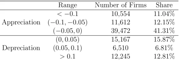
[Table 1 is to be here]
Transactions in the dataset have been classified into 18 different custom regimes.
Among all custom regimes, “ordinary trade” and “processing trade” (“processing
and assembly trade” and “processing with imported materials trade”) account for
more than 90% of total trade values in each year. Under the “processing and
assem-bly trade regime”, a domestic Chinese firm is offered payment-free raw materials
and parts by its foreign trading partners, and the firm has to sell its products to
the same foreign trading partner after local assembly. Similarly, although firms
un-der “processing with imported materials” can choose their import/export trading
partners, they still differ from firms exporting under the “ordinary trade” regime,
since their products must comply with certain known standards.14 These features
14
of the “processing trade” regime make the influence of exchange rate changes
neg-ligible on import and export quality for firms operating under this regime. As
such, our main regressions only focus on firms exporting under “ordinary trade”
regime.15
3.1.2. Firm-Level Production Data
Although the Chinese Customs trade dataset provides detailed information on
firm-product-destination level trade transactions, it does not contain
production-side information. The Annual Surveys of Industrial Production (ASIP) dataset
provides firm-level production information. This dataset reports detailed
infor-mation on the three major accounting statements for comprehensive state-owned
enterprises (SOEs) and non-SOEs with annual sales exceeding 5 million RMB
(which is roughly US ✩770,000). During the sample period 2000-2006, the
num-ber of firms contained in the dataset varies between 162,885 and 301,961. These
recorded enterprises account for more than 90% of total industrial output and over
70% of total industrial employment in 2004 (Brandt et al., 2012). The dataset
al-so reports comprehensive key financial variables, such as firm-level gross output,
capital stock, wage rate, material input costs, employment etc. The information
helps to control for firm-level factors which might affect the quality of products.
In order to use both the firm-level trade and production information, a key
step is to match the ASIP dataset with the Chinese Customs dataset. Although
both datasets provide firm identifers, these identifiers are not common across the
data sets. As such we cannot match the two datasets by firm identifer. Following
15
Upward et al (2013), we match the two datasets by using the firms’ name and
establishment year. Table 2 reports the matching results.
[Table 2 is to be here]
Table 2 indicates that in the matched sample, the total number of exporters
and importers accounts for 30.87% and 28.82% of the total exporters and importers
in the Customs dataset, respectively. The total export and import values in the
matched sample account for 24.63% and 21.55% of the total export and import
values recorded in the Customs dataset, respectively.16
3.1.3. Country Level Macro Data
The exchange rate is a key variable in this paper, which is obtained from
Penn World Table (PWT7.1). The Penn World Table (PWT thereafter) provides
bilateral nominal exchange rates, which are pegged to US dollar; we transform
these into Chinese RMB against foreign currency. We combine this macro-level
dataset with our previous matched sample using the country code available in both
datasets. Note that the PWT does not contain all countries that Chinese firms
traded with. Hence, combining the marco and micro data further decreases the
sample size. Detailed matched results are reported in Panel C of Table 2.
Results indicate that after combining the exchange rate information with our
matched sample, the number of exporting destinations and importing countries
falls to 125 import countries and 155 export countries. The number of trading firms
(importing and exporting), traded varieties and values do not change much. This
16
implies that those countries not contained in the PWT are not important trade
partners with China. In addition, in a subsequent regression we use consumer price
indices (CPIs) to adjust the firm-level nominal exchange rate to a real exchange
rate to check the robustness of our results. The CPIs in different countries are
taken from the International Financial Statistics (IFS).
3.2. Main Variables
3.2.1. Quality Measure
Following Khandelwal (2010) andHallak and Sivadasan (2013), this study
de-fines ‘quality’ as any attribute which raises consumer’s demand other than price.
That is, according to the utility function (1), given price, increases in the
qual-ity measure qc help to increase demand in country country c. Given the utility
function, quality can be inferred from the observed price and demand.
Follow-ing Khandelwal et al. (2013), traded “quality” of product k shipped to (imported
from) destination country (sourcing country) c by firm f in year t is denoted as
qf kct, and it satisfies the following demand function:17
xf kct =qf kctσ−1pf kct−σ Pctσ−1Yct (13)
wherexf kct denotes the demand for product k in destination cat year t, exported
by firmf. PctandYct are the price index and aggregate income of countrycin year
t, respectively. Taking logs of both sides of equation (13), and rearrange terms we
get:
ln(xf kct) +σln(pf kct) =ϕk+ϕct+εf hct (14)
17
where ϕk denotes a product fixed effect, which captures the difference in prices
and demand across different product categories arising from inherent product
spe-cific characteristics other than quality. ϕct is the country-year fixed effect, which
controls for the influence of the aggregate price level, Pct, and aggregate income,
Yct, on product’s price and demand. We regressln(xf kct) +σln(pf kct) on the
prod-uct fixed effect, country-year fixed effect, and a quality measure represented by:
ˆ
qf kct =
ˆ
εf kct
σ−1. The intuition behind this approach is that conditional on a price, products with high quality tend to have higher demand.
A crucial step in obtaining the quality measure is to find the value of the
e-lasticity of substitution, σ. In the literature, researchers adopt different methods
and data to estimate the value of σ. This enables us to construct quality
mea-sures without estimating the demand equation. After surveying a large number
of gravity-based estimates of Armington elasticity of substitution, Anderson and
Van Wincoop (2004) conclude that a reasonable range of σ is between [5,10]. In
our basic estimation, we adopt the lower bound value for the elasticity of
substi-tution, i.e., σ = 5. As a robustness check, we also take the upper bound value of
elasticity of substitution, σ = 10. In addition, we also try an alternative measure
of elasticity of substitution, which is estimated by Broda et al. (2006) at the HS
3-digit level for all Chinese exports, to construct quality measures.18
3.2.2. Firm-Level Effective Exchange Rates
A large macro-economics literature investigates the impact of exchange rate
movements on aggregate outcomes. For instance, Kenen and Rodrik (1986),
Las-trapes and Koray (1990), Hooper and Kohlhagen (1978), Baxter and Stockman
18
(1989), Branson and Love (1988), Campa and Goldberg (1995, 2001), and
Gold-berg et al(1999) investigate the influence of exchange rate changes on country-level
economic variables. Nucci and Pozzolo (2010), Chatterjee et al. (2013), Ekholm
et al.(2012),Berman et al. (2012) analyze effects at the industry-level. Typically,
in these studies the aggregate effective exchange rate is constructed by summing
up the weighted bilateral exchange rate between different trade partners, where
the weights are the bilateral trade shares. This methodology, while appropriate
for constructing aggregate effective exchange rates is not suitable for our firm-level
analysis. Clearly, movements of the aggregate effective exchange rate cannot reveal
the heterogeneity in firm-level effective exchange rate changes. We therefore
con-struct the firm-level effective import exchange rate based on firms’ import shares
in the base year from each sourcing country as follows:
EERf t = n X
c=1
δf c0ln(ERct/ERc0) (15)
where EERf t denotes the effective import exchange rate faced by firm f in year
t. ERct and ERc0 are the nominal exchange rate between Chinese Yuan and
the currency of country c in year t, and in the base year, respectively.19 δ
f c0
denotes firm f’s import share from the sourcing country c in the base year.20
Since we focus on firm-level quality upgrading through an import mechanism, we
use bilateral import shares as the weight instead of bilateral export shares. Based
on the definition in equation (15), an increase inEERf t implies a depreciation in
19
In this research, we take the initial year of the sample (2000) as the base year.
20
the firm-level effective import exchange rate.
We calculate the fluctuations of effective import exchange rate at firm-level
be-tween 2000-2006 according to equation (15). The empirical distribution is reported
in Table 3.
[Table 3 is to be here]
Table 3 shows that firm-level effective import exchange rate changes exhibit a wide
dispersion. This is attributed to the wide variations in sourcing partners across
firms. In our sample, 64.50% of firms experience effective import exchange rate
appreciations, and the rest experience effective import exchange rate depreciations.
3.2.3. Other Control Variables
In the regressions, we also control for a series of firm-level characteristics to
exclude their impact on firms’ product quality choice. First, we control for
firm-level productivity, since firm-firm-level productivity has been shown to be positively
related to firm-level product quality (Berman et al., 2012; Verhoogen, 2008).21
Second, following Bernini and Tomasi (2015), we proxy firm size using the log
number of employees working in each firm. We also control for the capital
in-tensity measured as the log values of tangible assets per employee. In general,
firms with higher capital intensity and larger size are more likely to adopt more
advanced technologies and produce higher quality products. Lastly, we followBas
and Strauss-Kahn (2015) and incorporate the number of imported varieties as an
explanatory variable. Table 4 reports descriptive statistics for our main variables.
[Table 4 is to be here]
21
4. Exchange Rate Fluctuations and Export Quality
In this section, we test Proposition 1 by empirically estimating the impact
of effective import exchange rate changes on firm-level export quality. In what
follows, we first conduct the benchmark regression. Second, we investigate the
heterogeneous effect of exchange rate changes on export quality across firms with
different productivities. Lastly, we conduct a series of robustness checks.
4.1. Benchmark Regressions
According to our model, an appreciation in the firm-level import exchange rate
leads firms to import higher quality intermediate inputs. Higher quality
interme-diates improve the quality of exported products. As such, Proposition 1 predicts a
negative correlation between the firm-level effective import exchange rate, EER,
and the firm-level export quality (EER increase means an import currency
appre-ciaiton). We test this prediction by running the benchmark regression:22
qf kctex =β0+β1EERf,t−1 +λXf,t−1+ηf kc+ηt+ζf kct (16)
where qex
f kct represents the quality of product k exported to country c by firm f
in year t. EERf,t−1 is firm i’s effective import exchange rate in year t−1, which is calculated according to equation (15). Xf,t−1 is a vector of time-varying at-tributes of firmf in yeart−1, containing firm-level productivity, capital intensity,
22
and firm size. ηf kc and ηt are the firm-product-destination fixed effects and year
fixed effects, respectively. The former captures the impact of time-invariant
firm-product-destination attributes on firm-level exported quality (e.g. distribution
costs, trade costs, etc.), while the latter captures the influence of macro shocks
on firm-level exported quality. ζf kct is the error term including all unobservable
factors affecting export quality.
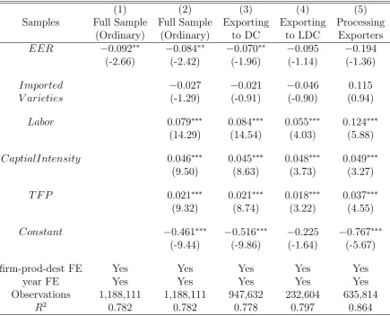
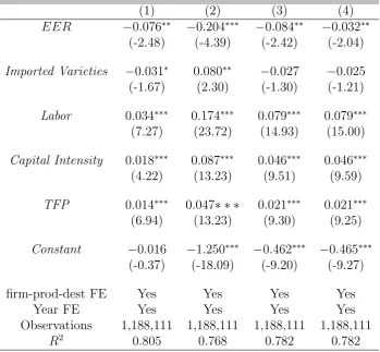
[Table 5 is to be here]
In column 1 of Table 5, we run regression (16) by excluding all control variables
but the fixed effects. The result shows that a 10% import currency appreciation
(a decrease in EER) will increase firm-level export quality by about 0.84%. In
column 2, we add more control variables in the regression, but the estimated effect
of an import currency appreciation remains unchanged.
We next divide our sample into two subsamples, one containing observations
exporting to developed countries, and the other containing observations
export-ing to developexport-ing countries. Developed countries are defined by the World Bank
as countries with per-capita GNIs above $9,760 in 2007 using the Atlas
conver-sation factor, while countries whose per-capita GNIs below $9,760 are classified
as developing countries. Columns 3 and 4 report export quality responses to
im-port exchange rate changes for observations exim-porting to developed and developing
countries, respectively. The results demonstrate a heterogeneous response of
ex-port quality in developed and developing countries.
In column 5, we run the regression for firms engaged in processing trade. The
result indicates that import exchange rate changes have a negative but statistically
Greenaway et al.(2008), who find that firms engaged in processing trade in China
are usually multinational firms (MNEs). Greenaway et al. (2008) conjecture that
MNEs can internalize exchange rate fluctuations and hence minimize the effects of
exchange rate movements in a number of ways, e.g., varying the speed of payments,
hedging foreign exchange transactions across countries, etc.
4.2. Heterogeneous Effects
Existing evidence suggests that firms exhibit heterogeneous reactions in
re-sponse to exchange rate changes. For example, Bernini and Tomasi (2015) and
Chen and Juvenal (2016) argue that firms exporting high quality products have a
lower exchange rate pass-through. Berman et al. (2012) and Li et al. (2015) both
document that more productive firms respond more to exchange rate movements
in their F.O.B export price, and Amiti et al. (2014) demonstrate that exchange
rate pass-through is decreasing in firm-level import intensity and export market
share.
In this section, we extend the results in Table 5 examine how firm-level
produc-tivity affects firm-level quality upgrading in response to an import appreciation. In
order to investigate the role that productivity plays, we add an interaction term
of firm-level productivity (TFP) with the effective import exchange rate to our
benchmark specification:
qexf kct =β0+β1EERf,t−1+β2EERf,t−1×T F Pf,t−1+λXf,t−1+ηf kc+ηt+ζf kct (17)
where T F Pf,t−1 is the productivity of firm f in year t−1. Our primary produc-tivity measure is estimated following Levinsohn and Petrin (2003). Designated
productivity measures, such as using Olley and Pakes (1996) (OP method) and
OLS methods,23 and re-estimate regression (17). β
2 captures the heterogeneous
export quality reaction to import exchange rate changes. The estimator results
from specification given by equation (17) are reported in Table 6.
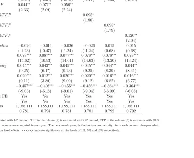
[Table 6 is to be here]
Column 1-3 in Table 6 reports the estimate results from specification (17)
by using productivities estimated from LP, OP and OLS methods, respectively.
All productivity measures are in levels. The results in column 1-3 indicate that
although exported quality is increasing in response to an import exchange rate
appreciation, quality upgrading declines as firm-level productivity increases. These
results suggest that more productive firms upgrade their exported quality at slower
rates relative to less productive firms.
As an additional check on this conclusion, in Column 4 - 6, we estimate
specifi-cation (17) using productivity percentiles instead of the levels. Specifically, we
in-teract the import exchange rate with different bins constructed from the estimates
of firm-level productivity. We construct dummy variables for exporters belonging
to each percentile category based on their own productivity and the distribution of
productivity by industry and year. We next interact percentile dummies with
im-port effective exchange rates. The bottom bin is chosen as the reference group. As
before, our results show that firms with higher productivity upgrade their
export-ed quality less than firms with lower productivity in response to an appreciation.
Specifically, firms with the highest 10% productivity increase their export quality
23
1.2% less than firms with the lowest productivity in our sample. In contrast, the
difference is only 0.95% between firms with productivity belonging to the top 50%
percentile and the firms with the lowest productivity.
The results reported in Table 6 are consistent with Proposition 1. The
intu-ition is that more productive firms export higher quality products. In response to
an import appreciation, these more productive firms cannot upgrade their
export-ed quality as much as less productive firms, as the quality transferring between
intermediates and final outputs becomes harder when initial quality is higher.24
Another possible explanation for this result is that high productive firms use high
quality intermediates. If they have used the best intermediates, there is no room
for them to further upgrade their export quality.25
4.3. Robustness
In the previous section, the empirical results show that an import currency
appreciation will lead firms to upgrade the quality of their exports to developed
markets, and this quality upgrading slows as firms become more productive. In
this section, we conduct a series of robustness checks to confirm our empirical
findings. First, we check if our results are driven by missing variables or sample
selection bias. Second, we investigate whether our results are robust to alternative
measures of quality and the effective exchange rate. Third, we examine whether
our results hold for different subsamples based on firm-level characteristics, to
24
According to our model, whenα <1, the quality transferring exhibits diminishing returns.
25
different standard error clustering methods, and after controlling for different fixed
effects. Lastly, we check our basic results by using a difference-in-difference (DID)
approach.
4.3.1. Missing Variables and Sample Selection
It is plausible that if a firm imports from the same country as it exports to,
the influence of exchange rate movements on this firm will be somewhat offset.
Similarly, import tariff could also affect firm-level export price and quality, i.e.
Bas and Strauss-Kahn (2015). Without controlling for the exchange rate in the
destination country and import tariffs cause a missing variable issue. Furthermore,
our sample contains only firms with positive imports,26which might cause a sample
selection issue. We estimate the benchmark regression by adding more controls
and an inverse Mill’s Ratio to alleviate the missing variable issue and sample
selection bias. These results are reported in Table 7.
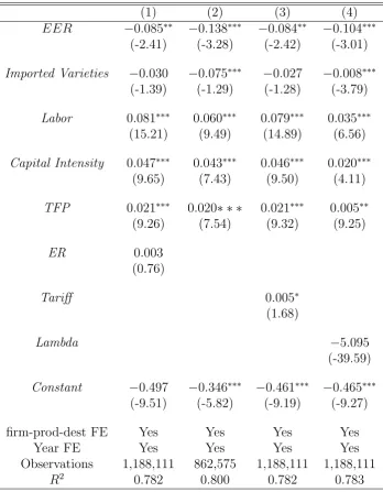
[Table 7 is to be here]
Column 1 of Table 7 reports the results after controlling for the bilateral
ex-change rate between China and export destinations. In column 2, we drop
ob-servations if the final product is exported to the same country that intermediate
inputs are imported from. Specifically, if a firm exports to countries A, B and
imports from countryA, we will only keep exports to country B in our regression.
Both column 1 and column 2 aim to avoid exchange rate movements in the
des-tination and sourcing countries might offset each other. Results of controlling for
26
import tariffs are reported in column 3. Column 4 reports the results of controlling
for firm-level self-selection into import.27 Results demonstrate that firms upgrade
their export quality in response to an increase in the effective import exchange
rate.
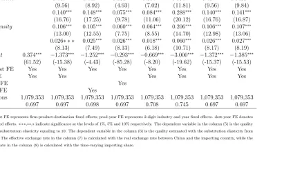
4.3.2. Different Measurements
To alleviate the concern that our quality and effective exchange rate measures
are biased, we construct an alternative quality measure by letting the elasticity
of substitution elasticity equal to 10,28 and use regression (14) to estimate export
quality. We also followBas and Strauss-Kahn (2015), and rely on the elasticity of
substitution at the HS 3-digit product level estimated by Broda et al. (2006) to
construct another quality measure. With these two alternative quality measures,
we run the benchmark regression (16) again. The results are reported in the
column 1- 2 in Table 8, and suggest that our results are not sensitive to which
quality measure we use, i.e., changes in the import effective exchange rate tend
to have a statistically significant effect on firm-level export quality, with import
currency appreciations leading to quality upgrades.
Countries also differ in their inflation rate. Without deflating exchange rates
by inflation, our measured effective import exchange rate is nominal. FollowingLi
27
A firm’s import decision usually relies on its productivity, export values and number of varieties. High productivity firms are more likely to import, while firms export more in terms of either extensive or intensive margins are more likely to use foreign materials. Therefore, the selection equation is set as: Dimpf t =γ1T F Pf,t−1+γ2EXPf,t−1+γ3V arietyf,t−1, whereDf t is a dummy variable which takes value 1 if firmf chooses to import in yeart, and 0 otherwise.
EXPf,t−1 and V arietyf,t−1 denote firm-level aggregate values and number of varieties in year
t−1.
28
et al. (2015), we use the CPI in each country as the deflator to construct the real
effective exchange rate as:
EERr f t=
n X
c=1
δf c0ln(
ERct
CP ICHN,t
/ERc0 CP Ict
) (18)
where EERr
f t denotes the real import effective exchange rate. CP ICHN,t and
CP Ict is the consumer price index in China and country c, respectively. We
re-estimate regression (16) using the real effective import exchange rate, and we
continue to find that import currency appreciations are associated with subsequent
improvements in exported quality. The result is shown in column 3 of Table 8.
Lastly, when we calculate the effective import exchange rate, the import share,
δf c0, is fixed. However, this share would vary by year: firms import more from
countries whose currency depreciates more relative to the Chinese Yuan. In column
4 of Table 8, we substitute δf c0 by δf ct to construct firm-level effective import
exchange rate and re-estimate regression (16).29 We continue to find that firms
upgrade their quality when facing an effective import appreciation.
[Table 8 is to be here]
4.3.3. Different Subsamples, Clustering and Fixed Effects
Another concern is that multiproduct firms may behave differently from single
product firms.30 A multiproduct firms can adjust its product mix in response to
shocks (Bernard et al.,2011). Also market size and degree of market competition
29
We notice that the variable import share cause an endogeneity issue. Here we only want to test whether our results are robust to different measures of import exchange rate.
30
determine multiproduct firms’ export mix (Mayer et al.,2011). When a
multiprod-uct firm ceases prodmultiprod-uction of a prodmultiprod-uct far from its core competence, demand for
its core competence products may increase. This cannibalization effect can cause
a pseudo quality increase in the firm’s core competence product.31 To address the
concern that the exported quality changes are driven by this pseudo quality change
in multiproduct firms, we estimate our benchmark regression (16) by keeping only
single product firms. This result is reported in column 1 of Table 9. The negative
(and significant) sign on the import exchange rate change implies that an import
currency appreciation increases the exported quality of single product exporters
as before.
One more concern might be our exclusion of firms engaged in processing trade.
That is as discussed in the data description section (section 3.1.1), we only keep
firms engaged in ordinary trade in our sample. However, notice that in response to
exchange rate fluctuations, a firm may find it profitable to switch from the ordinary
trade regime to the processing trade regime, or vice versa. In addition, firms’ entry
and exit from exporting markets in response to the movements of exchange rate
also might bias our estimation.32 Although Bas and Strauss-Kahn (2015) claim
that the trade status of Chinese exporters is stable over time,33 the entry and
exit rate from exporting market is non-trivial in our data. We therefore estimate
the benchmark specification with a subsample in which firms continuously export
31
The market cannibalization effect changes the demand of a particular product in a market. The demand changes will be attribute to quality changes if the cannibalization effect is not taken into account of.
32
However,Greenaway et al.(2008) find that exchange rate movements have a trivial effect on UK manufacturing firms’ entry probability.
33
under the ordinary trade regime throughout the 2000-2006 period. The result is
reported in column 2 of Table 9. Again we find a negative and significant coefficient
for EER, which is consistent with our benchmark regression results.
Another issue arises with respect to standard error clustering (Cameron et al.,
2011), since our dependent variable is at firm-product-destination level, and the
main explanatory variable is at firm level. Moulton (1990) shows that regressing
an individual level variable on more aggregate variables could induce a downward
bias in the estimation of the standard error. In order to address this possible
bias, we re-estimate the benchmark specification, and cluster the standard errors
at the HS 6-digit level (column 3); country level (column 4); product-country level
(column 5); and product-firm level (column 6), respectively. The results shown in
Table 9 are virtually unaffected by the method of clustering the standard errors.
Industry shocks may also force firms to switch their production from one
indus-try to another, or change their product quality. Indeed, in our sample 7.4% firms
changed their production at least once. To control for industry annual shocks, we
replace year fixed effects by industry-year fixed effects. At the meanwhile,
unob-served annual macro shocks in different destinations might affect firm-level export
quality decisions, e.g., a financial crisis in a particular destination could dampen
local consumers’ preference to high quality products. Therefore, we control for
country-year fixed effects.
The results in column 7 and 8 demonstrate that even after controlling for
industry-year and country-year fixed effects, we still obtain a negative and
sta-tistically significant coefficient on EER, further confirmation of our benchmark
[Table 9 is to be here]
4.3.4. DID Estimation
Lastly, it might be argued that there are omitted macro variables in our
bench-mark regression, which makes the casual relationship between import exchange
rate movements and export quality questionable. For instance, some unobserved
macro variables might cause a quality upgrading trend among all Chinese
exporter-s. Given the fact that more than 60% Chinese exporters experience effective import
appreciations during 2000-2006, the casual relationship we examined above could
be a pseudo relationship without controlling for export quality trends. In order to
alleviate this concern, we notice that the export quality of firms without imports
should not be affected by import exchange rate changes. This feature makes firms
not importing intermediates an ideal control group; firms with positive
interme-diate imports belong to the treated group. With the two groups of exporters, we
attempt to conduct one more robustness check by employing a strategy similar to
a difference-in-difference approach, where exporters with- and without-imported
intermediates belong to the treated and control groups, respectively.34 In this way,
we can exclude the impact of unobservable quality trends on our results.
For simplicity, we call firms that simultaneously engage in export and import
as “two-way exporters”, and firms only export as “one-way exporters”. As shown
in Table 10, 34.3%−42.7% of firms exporting under ordinary trade regime are two-way exporters during 2000-2006. These two-two-way exporters account for 84.8%−88% of total export values each year.
34
[Table 10 is to be here]
With the two-way and one-way exporters in our sample, we estimate the
fol-lowing DID specification:
qex
f kct =γ0+γ1EERf,t−1+γ2EERf,t−1T wowayf+γ3T wowayf+ζf kc+ζt+εf kct (19)
where, T wowayf is dummy variable, which takes value 1 if firm f is a two-way
exporter, 0 otherwise. All other variables have the same definitions as in
equa-tion (16). Since two-way exporters can switch to higher quality intermediates in
response to an import appreciation, which in turn, increases their export quality,
we expect the coefficient of the interaction term, γ2, to be negative. Note that
during the sample period, firms may switch from two-way exporters to one-way
exporters, or vice verse. It is problematic to define the switchers as either two-way
or one-way exporters. Hence, avoid the possibility that switchers contaminating
our results, we keep only firms maintaining their status, two-way or one-way
ex-porters, throughout their life span. It should be pointed out that the dummy
variable twowayf will be dropped from the estimation when we include a control
for firm-product-country fixed effect, as in our sample no firm switches its status.
These results are reported in Table 11.
[Table 11 is to be here]
In columns 1-3 of Table 11, we use the firm-level effective import exchange rate
defined by equation (15). In column 1 and column 2, export quality is estimated
following Khandelwal et al.(2013) by setting the elasticity of substitution to be 5
et al. (2006). The coefficient γ2 are negative and significant throughout column
1-3. This confirms our earlier results that in response to an import appreciation,
export quality increases for two-way exporters.
In columns 4-5, export quality is estimated as in column 1 (the elasticity of
substitution has been set to 5). In column 4, we use the firm-level real exchange
rate as given in equation (18). In contrast, in column 5, the firm-level nominal
exchange rate is constructed by using equation (15), but we use the initial year’s
import share (substitute δf ct by δf ct0). The estimated coefficient γ2 in columns
4-5 remain negative and statistically significant. All these results suggest that in
response to an import appreciation, firms with imported intermediates tend to
upgrade their export quality. This is again consistent with our benchmark results.
In the next section, we further examine the impact of effective import exchange
rate changes on firm-level imported quality.
5. Exchange Rate Fluctuations and Import Quality
In the last section, we documented a casual effect of import exchange rate
movements on firm-level export quality. In this section, we examine the impact of
import exchange rate changes on firm-level import quality. If an exporter switches
to higher quality intermediate inputs in response to an import appreciation, it
would confirm the mechanism proposed in our model.
We first investigate the impact of import exchange rate changes on firm-level
import price and sophistication. The specification we estimate for imported price
is as follows:
where U Vf kct represents the unit value of intermediate k (at HS 6-digit level)
imported from sourcing country c by firm f in year t. RERk,t−1 measures the nominal exchange rate between China and the sourcing country c in year t−1. Notice the difference between RERk,t−1 and EERf,t−1. The former is country specific, while the latter is firm specific. An increase in RERk,t−1 indicates a depreciation in the domestic currency (Chinese yuan in our case). Df kc and Dt
separately capture the firm-product-country fixed effect and year fixed effect. εf kct
is the error term. Note that all variables are in levels (rather than first difference),
and hence, the estimated coefficients can be treated as capturing the long term
response of import unit values to changes in the bilateral exchange rate. Following
Chen and Juvenal(2016), we assume that the exchange rates are exogenous to the
pricing decisions of individual firms given the disaggregation of the data.
To test the impact of import exchange rate movements on firms’ import
so-phistication, we estimate the following specifications proposed byBas and
Strauss-Kahn (2015):
Sophisticationf t=λ0+λ1lnEERf,t−1+Df +Dt+ǫf t (21)
where Sophisticationf t denotes the import sophistication of firm f in year t. As
inSchott(2008), firm-level import sophistication is measured by the firm’s import
as before.35 Since firm specific characteristics and macro shocks might affect firms’
sourcing country decision, we also include firm fixed effect,Df and year fixed effect,
Dt, in the regression.36
The coefficients of interest in regression (20) and (21) are α1 and λ1,
respec-tively. The coefficient α1 is expected to be positive, while the coefficient λ1 is
expected to be negative. A positive α1 implies that an decrease in EER (i.e.,
an appreciation in the domestic currency) will lead to a lower import price. In
contrast, a negative λ1 implies that a decrease in EER (an appreciation in the
import exchange rate) increases firm-level import sophistication. Our results are
reported in Table 12.
[Table 12 is to be here]
Panel A in Table 12 reports the results for import price (equation 20). We
begin with a sample containing firms exporting under the ordinary trade regime.
The result in column 1 of Panel A shows a positive α1, which implies that an
appreciation leads to a decline in import unit price. It is arguable that during
2000-2006, a surge in raw materials and energy prices might drive this result in
column 1. Hence, we estimate (20) again by excluding observations of importing
raw materials and energy.37 The results are shown in column 2 of Panel A. The
result in column 2 is quite similar to that reported in column 1. This suggests
35
Note that in the unit value regression, we adopt bilateral exchange rate as the explanatory variable, while in the sophistication regression, we use firm-level import exchange rate as explana-tory variable. The reason is that the former, import unit value, is at the firm-product-country level, and hence bilateral exchange rate is more straightforward, while the latter, sophistication, is at firm-level, we have to use the firm-level import exchange rate as the independent variable.
36
We use only the Customs data to estimate regression (20) and (21).
37
that the estimated positive α1 is not caused by a surge in prices of raw materials
and energy. Also notice that α1 < 1, which implies an incomplete pass-through
of exchange rates on import price, a result found by many earlier researchers (e.g.
Campa and Goldberg, 2005;Goldberg and Knetter,1997; Gopinath and Rigobon,
2008, etc.).
In columns 3 and 4 of Panel A, we divide imported intermediates from
de-veloped countries and developing countries, and run the regression (20) for each
subsample, respectively. The definition of developed and developing countries are
the same as before(see subsection 3.1). The results in column 3 indicate that a
10% appreciation corresponds to a 4.79% decrease in the price of imports from
de-veloped countries. This influence is twice the import price decrease in developing
countries (2.56%), and seems to contradict evidence in Chen and Juvenal (2016)
andBernini and Tomasi (2015), who both find that firms exporting higher quality
products, tend to exhibit smaller pass-through. However, since developed
coun-tries usually produce higher quality intermediates than developing councoun-tries do, (
ignoring importers switching to higher quality intermediates), we should expect a
smaller decline in import prices falling of intermediates imported from developed
countries. Our model predicts that quality upgrading is harder for firms exporting
(importing) higher quality products (intermediates) if the quality transferring
be-tween intermediates and final products exhibits diminishing returns. Therefore, all
other things equal, in response to an import currency appreciation, firms
import-ing from developimport-ing countries upgrade their imported intermediate quality more
developing countries decreasing less than that in developed countries.38
Results in Panel B of Table 12 investigate the effect of firm-level import
ex-change rate ex-changes on firms’ import sophistication. In columns 1-2, we do not
control for year fixed effects, while in columns 3 and 4 we control for firm fixed
effects and year fixed effects. In addition, in columns 1 and 3, we construct the
import sophistication measure using firms’ import share from developed countries,
in terms of values:
Sophistif icationf t =
Importing Values from Developed Countries Total Import Values
In columns 2 and 4, we construct the firm-level import sophistication using firms’
import share from developed countries, in terms of quantities:
Sophistif icationf t=
Importing Quantities from Developed Countries Total Import Quantities
All results demonstrate the pattern that when the domestic currency appreciates,
firms’ import share from developed countries increases. This is consistent with
increases in firm-level import sophistication in response to import appreciation.
In sum, Table 12 indicates that when the domestic currency appreciates,
firm-level import prices decrease, and more so for intermediates from developed
coun-tries, and that firm-level import sophistication increases.
38
5.1. Exchange Rate Fluctuations and Imported Products Quality
Although firms’ import price and sophistication exhibit patterns supporting our
quality upgrading story, we realize that import price changes in different sourcing
countries might not be driven by import quality changes, but rather by markup
changes. Also firms’ import sophistication increases might simply reveal that firms
begin importing more varieties from developed countries. In order to address these
concerns, we follow the steps used previously in the estimation of exported product
quality (see Section 4.3.2), in the construction of our imported intermediate quality
measures. These results are reported in Table 13.
[Table 13 is to be here]
In columns 1-4 of Table 13, import quality is estimated by using specification
(14) but here we replace export quantities and prices by import quantities and
prices. As before, the elasticity of substitution has been set to be 5. Column 1
regresses import quality on the import exchange rate. Columns 2-4 repeat the
regression in column 2, but with different fixed effects. Specifically, column 2
controls for product-country and year fixed effects; column 3 controls for
product-country and product-year fixed effects; and column 4 controls for
firm-product-country and country-year fixed effects, respectively. Results in columns
1-4 suggests that in response to an import appreciation, firm-level import quality
increases.
In column 5, we continue to estimate firm-level import quality using
specifi-cation (14) but we set the elasticity of substitution equal to 10. In column 6, we
follow the method used by Broda et al. (2006) to construct another import
coefficient on EERf,t−1.
In column 7, we use CPIs in each country to deflate the nominal exchange
rate and construct the effective real import exchange rate according to equation
(18). In column 8 we construct firmlevel import exchange rate as in columns 1
-6 by using specification (15), but replace the constant import share, δf ct0, by the
time-varying import share, δf ct. Again, the results suggest that firm-level import
quality increases with import currency appreciation, whether we consider nominal
or real exchange rates.
6. Conclusions
This paper examines the impact of exchange rate fluctuations, in particular,
firm-level import exchange rate fluctuations, on firm-level import and export
qual-ity. Our argument is that a decrease in firm-level import exchange rate (i.e. an
appreciation in the domestic currency) enables firms to upgrade their exported
product quality by buying higher quality intermediates, which they could not
af-ford before.
We first develop a theoretical model highlighting the role of exchange rates
in firm-level imported intermediates, and their export product quality decisions.
Following others (e.g. Rodrigue and Tan, 2016; Bas and Strauss-Kahn, 2015),
we assume a positive linkage between the quality of intermediate input and the
quality of final products. The model predicts that firm-level export product quality
increases in response to an import appreciation, which is achieved by switching to a
higher quality of imported intermediates. Furthermore, if the quality transferring
between the intermediate inputs and final outputs exhibits diminishing returns,