Multiphasic growth models for cattle

Interest in the modelling of animal growth is caused, besides interest in studying the biological phenomena themselves, by important economic implications growth has for animal breeders. A fit-ting model gives an opportunity to summarize im-portant growth characteristics (such as growth rate, earliness, daily gain, food conversion, mature body size and weight, length of the time interval between birth and maturity) into just a few model param-eters. These parameters can be used as a base of selection (e.g. Beltran, 1992; Mignon-Grasteau et al., 2000). Statistical analysis can also identify relations between growth curve parameters and important production and reproduction traits (e.g. de Torre et al., 1992; Menchaca et al., 1996; Hyánková et al., 2001). Frequently used are also allometric mod-els (e.g. Zeger et al., 1987; Koops and Grossman, 1991b).

Classicalgrowth models1 _{assume that the}

postna-tal growth rate monotonically increases until certain age when it reaches maximum and then it monotoni-cally decreases and (asymptotimonotoni-cally) reaches zero. The corresponding growth curve is a smooth

mo-notonic sigmoidal curve with one inflection point (which corresponds to the maximum growth rate age) and an asymptote. The growth model often de-scribes a relation between live weight of an animal

y and its age t. Then the asymptote of the growth

curve is usually interpreted as the final weight of an adult animal.

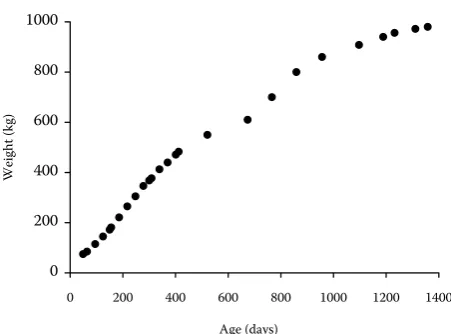
Observed growth data may reveal in some cases that the real growth is a more complex process than the above-mentioned classical model assumes. The growth data on Czech Pied breeding bulls in Figure 1 indicate that a multiphasic growth model with two classical phases could fit the data better than the classi-cal one. Multiphasic growth models were proposed by Koops (1986) and since that time multiphasic growth was examined in several species (chicken – Koops and Grossman, 1988; mouse – Koops et al., 1987; Kurnianto et al., 1999; Koops and Grossman, 1991a,b; pig – Koops and Grossman, 1991c; Japanese quail – Knížetová et al., 1995; allometric relations in rab-bits, fish and chicken – Koops and Grossman, 1993); for related papers see also Hyánek and Hyánková, 1995; Nešetřilová, 1998).

Multiphasic growth models for cattle

H. NEŠETŘILOVÁ

Czech University of Agriculture, Prague, Czech Republic

ABSTRACT: There are several ways of generalizing classical growth models to describe the complex nature of animal growth. One possibility is to construct a model based on a sum of several classical growth functions. In this paper, such multiphasic growth models for breeding bulls of the Czech Pied cattle based on the sum of two logistic functions are studied. The logistic function was chosen as a base for the models due to the relatively low degree of nonlinearity for the growth data. The paper describes three steps of constructing such a multiphasic growth model: in the first step a model with four unknown parameters is considered, in the second step the number of model parameters which are to be estimated is increased to five and in the third step a general model with six parameters is used. In each step, statistical properties of the considered model are checked. The residual variability of the best fitting model is on average approx. 8 times lower than the residual variability of classical Gompertz model which is often used by breeders to model cattle growth.

Keywords: multiphasic growth models; nonlinear regression; degree of nonlinearity; cattle growth; breeding bulls

METHOD

For the purpose of the study, data on body weight of 101 breeding bulls of the Czech Pied cattle were collected. Body weight was recorded from approx. 30 days up to (max.) 1 400 days of age. The weigh-ing interval was approx. 30 days, nevertheless it differed individually.

The observed growth data (Figure 1) suggest that a suitable multiphasic growth model could be con-structed either as a sum of two classical growth functions or as a change point model. In this paper, the first approach was considered and the mean

body weight of individual bulls was modelled as a

sum of two growth functions (corresponding to two “classical” growth phases). As possible candidates for the construction of such a multiphasic model were considered the following functions (which are used as the “classical” growth models):

Logistic

y = α (1)

1 + exp (β – γt)

Gompertz

y = α exp(–exp (β – γt)) (2)

Richards

y = α (1 + exp (β – γt))–1/δ ₍₃₎

Morgan – Mercer – Flodin

y = βγ + αtδ (4)

γ + tδ

Weibull type

y = α – β exp(–γtδ_{) (5)}

Among those models, Gompertz and Richards functions have often been used for cattle growth modelling.

Nešetřilová (2001) compared statistical prop-erties of functions (1) to (5) in classical models of growth data on the Czech Pied breeding bulls. Based on this study, two functions were considered for the construction of the multiphasic model, lo-gistic and Gompertz. Especially the lolo-gistic func-tion seemed to be a reasonable choice because of the low degree of nonlinearity. In this paper, the growth model based on the sum of two logistic functions is considered. For the model based on the sum of two Gompertz functions see Nešetřilová (2004).

The growth model which is a sum of two logis-tic functions has, in general, six parameters which have to be estimated from data. As the number of parameters was considered too high and as there

were some indications that parameter βcould be

the same for both growth phases, the growth model was constructed in three steps.

In the first step the assumption was made that

β₁ = β₂ (= β) and moreover its value was set fixed for

each animal. (This step was considered as prepara-tory and its purpose was to help set initial values for estimates in the second step.) This growth model referred to as LOGISTIC 4 had four parameters which were estimated from the observed data,

y = α1 + α2

1 + exp (β_fix – γ₁t_{) 1 + exp (βfix} – γ₂t)

(LOGISTIC 4) where: β_fix = the fixed numerical constant2

α₁, α₂ , γ₁, γ₂ = model parameters

In the second step, β was considered to be an unknown parameter and thus the corresponding

model LOGISTIC 5 had five parameters α₁, α₂, β,

γ₁, γ₂

y = α1 + α2

1 + exp (β – γ₁t) 1 + exp (β – γ₂t₎

(LOGISTIC 5) The most general model was LOGISTIC 6 with

six parameters α₁, α₂, β₁, β₂, γ₁, γ₂

y = α1 + α2

1 + exp (β₁ – γ₁t) 1 + exp (β₂ – γ₂t)

(LOGISTIC 6)

In these models α₁ (α₂) represents the asymptote

of the first (second) growth phase, γ₁ (γ₂) growth

rate in the first (second) growth phase and α₁ + α₂

is the asymptote of the resulting growth curve

(lim y(t) = α₁ + α₂). Parameters β (β₁, β₂) have no

straightforward biological interpretation.

Considered models are nonlinear regression models, thus their properties can be studied only in combination with data sets for which they are used. This is caused by the fact that the regression

2_{Choice of β was based on the fact that}

β = ln( α1 + α2 _–1)

y(0)

response surface can have different properties for different data sets (see Ratkowsky, 1983).

Two criterions were used to evaluate the good-ness-of-fit of a growth model. The first criterion was residual variability measured by residual

vari-ance s2

s2 ₌ S

n – p

where: S = S(ϑ) ∧ = the residual sum of squares of the parameter vector estimate, ϑ∧ = (∧

α₁,∧

α₂,∧ γ1,

∧

γ2) and/or

∧

ϑ = (∧

α₁,∧

α₂, β∧₁,∧ γ1,

∧ γ2) or

∧

ϑ = (∧

α₁,∧

α₂,β∧₁,β∧₂,∧ γ1,

∧ γ2) n = denotes the number of observations

p = the number of model parameters; (s2 _was preferred to S due to the unequal number of observations on individual animals)

The second criterion was the degree of “non-linearity” for a specific model/data combination because regression models with a low degree of nonlinear behaviour have preferable statistical

properties3 _{(see Ratkowsky, 1983).}

Nonlinearity of a model can be separated into two

components: intrinsic nonlinearity (associated with

geometric properties of the solution locus, with

its curvature) and parameter-effects nonlinearity

(associated with parametrisation of the model)4_.

It is strongly recommended to use close-to-linear models which have both the low intrinsic nonlin-earity and low parameter-effects nonlinnonlin-earity (for details see Ratkowsky, 1983; Zvára, 1989).

RESULTS AND DISCUSSION

The model LOGISTIC 4 (fixed β) was considered only as a preparatory step for the subsequent con-struction of more complex models. It helped to set initial estimates of parameters of the more com-plex model LOGISTIC 5 (β estimated parameter). Convergence to the final estimates was fast, also

due to the relatively low5 _{degree of nonlinearity of}

logistic models for the bull data (Tables 4 and 5).

Table 1 summarizes residual sums of squares S and

residual variances s2_{for bulls}6 _{from the considered}

group with maximum number of weight

determi-nations n. In the model LOGISTIC 6 (generally

β₁ ≠ β₂) residual variability, measured by the

re-sidual sum of squares S, further decreased. The

decrease in residual variability was marked in some

3_{Nonlinear regression models differ from linear regression models in this way: when the assumption of}

inde-pendent and identically distributed normal random errors is made, the least-squares estimators of linear model parameters are generally unbiased, normally distributed and have minimum variance while in the case of nonlinear models the least-squares estimators have these properties only asymptotically. Thus, the

estimators are generally biased and their properties (incase of a finite sample) are not known. The extent

to which a nonlinear model differs from a linear one (bias, degree of nonnormality, increase of estimator variability) can vary greatly for different nonlinear model/data combinations. Thus it is not possible to give a general recommendation as to how large the sample size must be so that the properties of a model are close to its asymptotic behaviour. Further, magnitude of an estimator bias and increase of the estimator variability are related to the degree of the “nonlinearity” of its distribution. Besides the advantages mentioned above (close-to-asymptotic behaviour), predicted response values y will have only a small bias and computational complexity and problem of the initial estimates of the parameter vector will also decrease.

4_{Intrinsic nonlinearity has an impact on the extent of bias of y predictions while parameter-effects nonlinearity may}

negatively influence the convergence to the least-square estimates of the model parameters. Parameter-effects nonlinearity may sometimes be decreased by suitable reparametrization of a model while intrinsic nonlinearity does not depend on parametrization.

5_{Degree of nonlinearity is considered low if it is bellow (F}

0.95(p, n – p))–1/2 (Tables 4–6).

6_{All models were constructed for individual animals.}

0 200 400 600 800 1000

0 200 400 600 800 1000 1200 1400

Age (days)

W

ei

ght

(k

g)

Table 1. Residual sum of squares S, residual variance s2 _{and number of observations n for individual growth curves}

in models LOGISTIC4 – LOGISTIC 6

Model LOGISTIC 4 LOGISTIC 5 LOGISTIC 6

Bull No. n S s2 _{S s}2 _{S s}2

1 28 2 768.67 115.36 1 910.87 83.08 1 901.29 86.42

2 26 3 699.60 168.16 3 032.28 144.39 1 535.16 76.76

3 32 4 791.18 171.11 4 469.94 165.55 2 388.79 91.88

4 32 6 563.31 234.40 3 742.67 138.62 3 382.83 130.11

5 32 13 199.93 471.43 4 910.81 181.88 4 863.76 187.07

6 26 3 215.13 146.14 3 192.24 152.01 3 186.29 159.31

7 25 3 766.67 179.37 1 570.39 78.52 1 262.94 66.47

8 27 2 380.48 103.50 2 330.78 105.94 2 272.14 108.20

Table 2. Parameter estimates and their asymptotic standard errors of the model LOGISTIC 4 (fixed β)

Bull No. Parameter α1 Parameter α2 Fixedβ Parameter γ1 Parameter γ2

estimate ASE* estimate ASE* estimate ASE* estimate ASE*

1 384.553 11.364 705.665 37.776 3.055 0.01221 0.00033 0.00306 0.00016

2 332.079 12.860 692.543 13.711 3.106 0.01600 0.00056 0.00432 0.00012

3 314.477 16.502 623.625 17.342 2.944 0.01367 0.00057 0.00403 0.00017

4 303.255 13.538 789.670 14.210 3.066 0.01630 0.00069 0.00445 0.00011

5 341.826 18.803 642.274 20.814 3.229 0.01617 0.00082 0.00441 0.00018

6 296.640 14.454 699.899 13.956 2.944 0.01405 0.00058 0.00390 0.00011

7 309.308 9.008 735.177 38.382 3.001 0.01751 0.00068 0.00327 0.00016

8 392.951 13.367 570.090 13.750 2.890 0.01280 0.00034 0.00374 0.00014

*asymptotic standard error

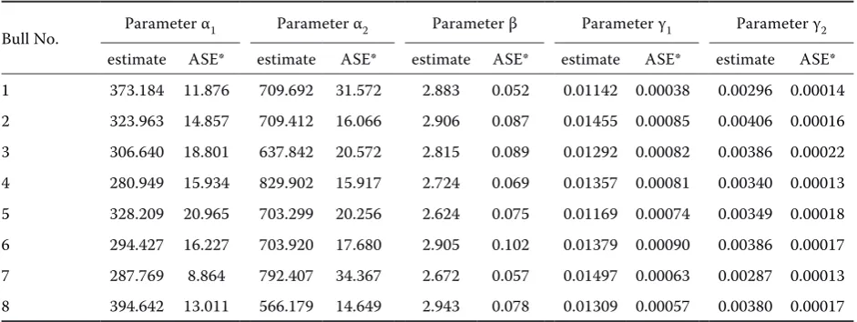
Table 3. Parameter estimates and their asymptotic standard errors of the model LOGISTIC 5 (estimate β)

Bull No. Parameter α1 Parameter α2 Parameter β Parameter γ1 Parameter γ2 estimate ASE* estimate ASE* estimate ASE* estimate ASE* estimate ASE*

1 373.184 11.876 709.692 31.572 2.883 0.052 0.01142 0.00038 0.00296 0.00014

2 323.963 14.857 709.412 16.066 2.906 0.087 0.01455 0.00085 0.00406 0.00016

3 306.640 18.801 637.842 20.572 2.815 0.089 0.01292 0.00082 0.00386 0.00022

4 280.949 15.934 829.902 15.917 2.724 0.069 0.01357 0.00081 0.00340 0.00013

5 328.209 20.965 703.299 20.256 2.624 0.075 0.01169 0.00074 0.00349 0.00018

6 294.427 16.227 703.920 17.680 2.905 0.102 0.01379 0.00090 0.00386 0.00017

7 287.769 8.864 792.407 34.367 2.672 0.057 0.01497 0.00063 0.00287 0.00013

8 394.642 13.011 566.179 14.649 2.943 0.078 0.01309 0.00057 0.00380 0.00017

animals but in others it was only so slight that the

residual variance s2_{, which penalizes the model for}

the number of parameters, increased. The com-parison of models LOGISTIC 5 and LOGISTIC 6 indicates that for some animals the parameter β might be the same for both growth phases but for others it is not true.

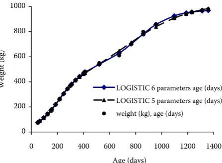
Point estimates of model parameters and their precision (characterised by asymptotic standard errors) for models LOGISTIC 4–LOGISTIC 6 are given in Tables 2–4. As expected, the precision of estimation decreased with the number of param-eters of the model but the drop was not fatal. This fact is related to the increase of nonlinearity (see below). The shape of growth curves LOGISTIC 5 and LOGISTIC 6 and their correspondence to data can be visually inspected in Figure 2.

The second criterion to evaluate the goodness-of-fit was a close-to-linear behaviour of a growth model. For its evaluation, measures of nonlinearity of considered model/data combinations in mod-els LOGISTIC 4–LOGISTIC 6 were computed (Tables 5–7). Nonlinearity is usually classified as high if the maximum of the corresponding measure exceeds

F_0.95(p, n – p))–1/2

where: n = the size of a data sample

p = the number of model parameters (see Zvára, 1989, p. 230)

A comparison of the level of nonlinearity in the models LOGISTIC 5 and LOGISTIC 6 is interesting in this respect. While in the model LOGISTIC 5 the intrinsic nonlinearity was low and the

parameter-effects nonlinearity exceeded F_0.95(p, n – p))–1/2 _only

0 200 400 600 800 1000

0 200 400 600 800 1000 1200 1400 Age (days)

Weight (kg) LOGISTIC 6 parameters age (days) LOGISTIC 5 parameters age (days) weight (kg), age (days)

Figure 2. Individual growth modelled by LOGISTIC 5 and LOGISTIC 6

Ta bl e 4. P ar am et er e st im at es a nd th ei r a sy m pt ot ic st an da rd e rr or s o f t he m od el L O G IS T IC 6 (e st im at e β1 , β2

Table 5. Degree of nonlinearity of the multiphasic growth model LOGISTIC 4 (fixed β) for data on Czech Pied bulls

Bull No. Average curvature Maximum curvature (F_0.95(p, n – p))–1/2

parameter effects intrinsic parameter effects intrinsic

1 0.7707 0.1211 2.1603 0.3218 0.6002

2 0.2067 0.0727 0.4300 0.1770 0.5958

3 0.4175 0.1037 1.0353 0.2729 0.6070

4 0.2113 0.0799 0.4894 0.2026 0.6070

5 0.3160 0.1077 0.6808 0.2673 0.6070

6 0.2667 0.0760 0.6378 0.1978 0.5958

7 0.5942 0.0972 1.6407 0.2359 0.5934

8 0.3167 0.0710 0.8092 0.1830 0.5980

Table 6. Degree of nonlinearity of the multiphasic growth model LOGISTIC 5 (estimate β) for data on Czech Pied bulls

Bull No. Average curvature Maximum curvature (F_0.95(p, n – p))–1/2

parameter effects intrinsic parameter effects intrinsic

1 0.6651 0.0394 2.2365 0.1176 0.6155

2 0.3010 0.0560 0.8620 0.1782 0.6103

3 0.5100 0.0736 1.5506 0.2394 0.6235

4 0.3032 0.0610 0.9401 0.2019 0.6235

5 0.4762 0.0730 1.3832 0.2367 0.6235

6 0.3243 0.0606 0.9540 0.1980 0.6103

7 0.5760 0.0420 1.9220 0.1332 0.6073

8 0.3298 0.0501 0.9899 0.1538 0.6130

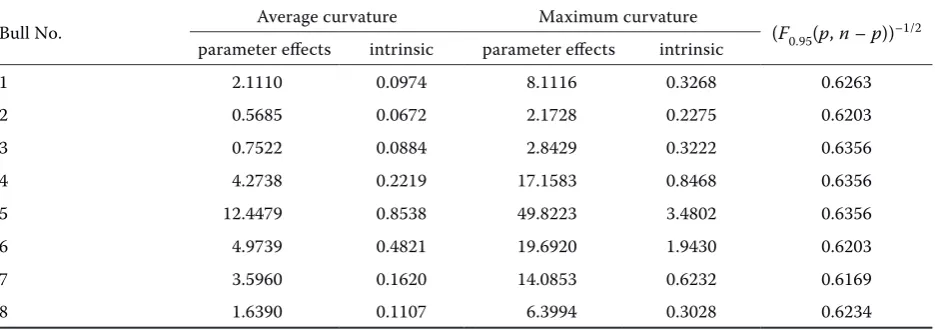
Table 7. Degree of nonlinearity of the multiphasic growth model LOGISTIC 6 (estimate β₁, β₂) for data on Czech Pied bulls

Bull No. Average curvature Maximum curvature (F_0.95(p, n – p))–1/2

parameter effects intrinsic parameter effects intrinsic

1 2.1110 0.0974 8.1116 0.3268 0.6263

2 0.5685 0.0672 2.1728 0.2275 0.6203

3 0.7522 0.0884 2.8429 0.3222 0.6356

4 4.2738 0.2219 17.1583 0.8468 0.6356

5 12.4479 0.8538 49.8223 3.4802 0.6356

6 4.9739 0.4821 19.6920 1.9430 0.6203

7 3.5960 0.1620 14.0853 0.6232 0.6169

8 1.6390 0.1107 6.3994 0.3028 0.6234

moderately, the intrinsic nonlinearity in the model LOGISTIC 6 was high and parameter-effects

non-linearity exceeded F_0.95(p, n – p))–1/2 _{considerably in}

estimates (Table 4). Thus, the model LOGISTIC 5 had better statistical properties than the model LOGISTIC 6 but the question if it was accepta-ble for the observed data was open. To answer it,

an asymptotic test for testing H₀ : β₁ = β₂ against

A : β₁ ≠ β₂ was performed (see Ratkowsky, 1983,

p. 138). The test, based on the change in the re-sidual sum of squares between models LOGISTIC 5 and LOGISTIC 6 for all considered animals, ended in rejection of the null hypothesis (α < 0.01).

Thus the general model LOGISTIC 6 with six

parameters α₁, α₂, β₁, β₂, γ₁, γ₂ should be considered

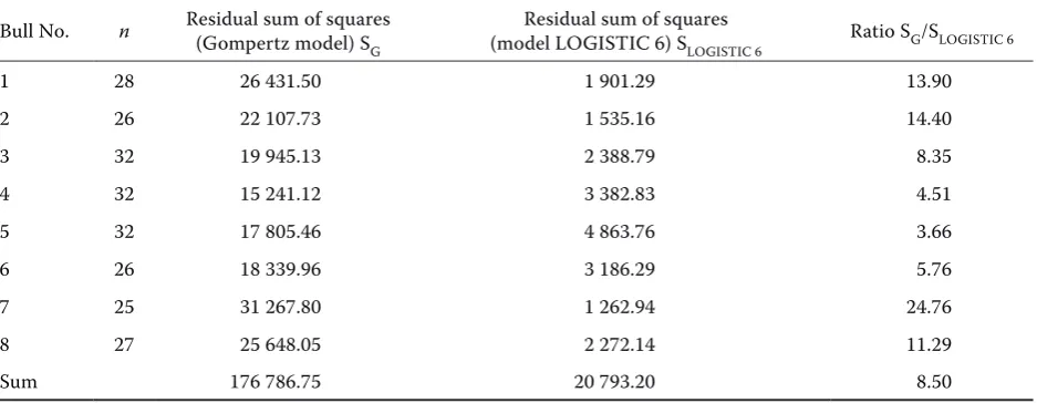
as adequate for the modelling of bull growth. To document the improvement of using this model in comparison with the classical Gompertz model, the residual variability for both models is presented in Table 8. For the same growth data, the multiphasic growth model LOGISTIC 6 has on average more than 8 times lower residual sum of squares than the Gompertz model which is often used to model cattle growth.

Efforts to find a growth model which fits the ob-served data as close as possible are justified by the fact that parameters of the growth model can be used for estimation of breeding value of an animal and for subsequent selection. Considering the impact breeding bulls have on production and reproduction traits in cattle subpopulations, further research on more appropriate growth models is desirable.

Acknowledgements

I would like to express my gratitude to Doc. RNDr. Karel Zvára, CSc., from Faculty of Mathematics and

Physics of Charles University in Prague, who was so kind to compute nonlinearity measures for my data. Standard software packages do not allow these com-putations and he used his own program to do so.

REFERENCES

Beltran J.J., Butts W.T., Olson T.A., Koger M. (1992): Growth patterns of two lines of Angus cattle selected using predicted growth parameters. J. Anim. Sci., 70, 734–741.

De Torre G.L., Candotti J.J., Reverter A., Bellido M.M., Vasco P., Garcia L.J., Brinks J.S. (1992): Effects of growth curves parameters on cow efficiency. J. Anim. Sci.,70, 2668–2673.

Fitzhugh H.A. (1976): Analysis of growth curves and strategies for altering their shape. J. Anim. Sci., 42, 1036–1051.

Hyánek J., Hyánková L. (1995): Multifázické růstové křivky. Živoč. Výr., 40, 283–286.

Hyánková L., Knížetová H., Dědková L., Hort J. (2001): Divergent selection for shape of growth curve in Japa-nese quail. 1. Response in growth parameters and food conversion. Brit. Poult. Sci., 42, 583–589.

Knížetová H., Hyánek J., Hyánková L., Dědková L. (1995): Matematické funkce a jejich využití při analýze růstu ve vztahu ke konverzi krmiva. [Závěrečná zpráva.] VÚŽV,Praha-Uhříněves.

Koops W.J. (1986): Multiphasic growth curve analysis. Growth, 50, 169–177.

Koops W.J., Grossman M. (1991a): Multiphasic analysis of growth curves for progeny of a somatotropin trans-genic male mouse. Growth, 55, 193–202.

Table 8. Residual sum of squares of the classical Gompertz model and the multiphasic logistic model LOGISTIC 6 and their ratio

Bull No. n Residual sum of squares _{(Gompertz model) S} G

Residual sum of squares

(model LOGISTIC 6) SLOGISTIC 6 Ratio SG/SLOGISTIC 6

1 28 26 431.50 1 901.29 13.90

2 26 22 107.73 1 535.16 14.40

3 32 19 945.13 2 388.79 8.35

4 32 15 241.12 3 382.83 4.51

5 32 17 805.46 4 863.76 3.66

6 26 18 339.96 3 186.29 5.76

7 25 31 267.80 1 262.94 24.76

8 27 25 648.05 2 272.14 11.29

Corresponding Author

Doc. RNDr. Helena Nešetřilová, CSc., Czech University of Agriculture, Kamýcká 129, 165 21 Prague 6-Suchdol, Czech Republic

Tel. +420 224 382 253, fax + 420 220 920 321, e-mail: [email protected] Koops W.J., Grossman M. (1991b): Multiphasic growth

and allometry. Growth, 55, 203–212.

Koops W.J., Grossman M. (1991c): Application of a mul-tiphasic growth function to body composition in pigs. J. Anim. Sci., 69, 3265–3273.

Koops W.J., Grossman M. (1993): Multiphasic allometry. Growth, 57, 183–192.

Koops W.J., Grossman M., Michalska E. (1987): Multipha-sic growth curve in mice. Growth, 51, 217–225. Kurnianto E., Shinjo A., Suga D. (1999): Multiphasic

analysis of growth curve of body weight in mice. Asian-Australs. J. Anim. Sci.,12, 331–335.

Menchaca M.A., Chase C.C., Olson T.A., Hammond A.C. (1996): Evaluation of growth curves of Brahman cattle of various frame sizes. J. Anim. Sci.,74, 2140–2151. Mignon-Grasteau S., Piles M., Varona L., de Rochambeau

H., Poivey J.P., Blasco A., Beaumont C. (2000): Genetic analysis of growth curves parameters for male and fe-male chickens resulting from selection on shape of growth curve. J. Anim. Sci.,78, 2515–2524.

Nešetřilová H. (1998): Růstové modely v chovu skotu. [Habilitační práce.] ČZU, Praha. 165 pp.

Nešetřilová H. (2001): Comparison of several growth models for the Czech Pied Cattle. Czech J. Anim Sci.,

46, 401–407.

Nešetřilová H. (2004): Criterions of selection of a regres-sion growth model (in Slovak). In: Kvantitatívne metódy v ekonómii. Nitra, FEM SPU. 141–145.

Ratkowsky D.A. (1983): Nonlinear Regression Modelling. Marcel Dekker, New York and Basel. 276 pp.

Zeger Scott L., Harlow S.D., Siobán D. (1987): Mathe-matical models from laws of growth to tools for bio-logical analysis: fifty years of Growth. Growth,51, 1–21.

Zvára K. (1989): Regresní analýza. Academia, Praha. 245 pp.