Bayesian models for sequential bidding and related theoretical topics

warwick.ac.uk/lib-publications

A Thesis Submitted for the Degree of PhD at the University of Warwick

Permanent WRAP URL:

http://wrap.warwick.ac.uk/108057/

Copyright and reuse:

This thesis is made available online and is protected by original copyright.

Please scroll down to view the document itself.

Please refer to the repository record for this item for information to help you to cite it.

Our policy information is available from the repository home page.

B A Y E S I A N M O D E L S F O R

S E Q U E N T I A L B I D D I N G

A N D R E L A T E D T H E O R E T I C A L T O P I C S

by

D u n c a n N o e l A t t w e ll

Dip.Statis.(Cantab), B.Sc., A.R.C.S.

Thesis submitted for the degree of Doctor o f Philosophy at the University of Warwick

D e p a r t m e n t o f S ta tis tic s U n iv e r s it y o f W a r w ic k

C O N T E N T S

S U M M A R Y ... iv

1. IN T R O D U C T IO N ...1

1.1 T h e Sequential B idding Problem ...1

1.2 S c h e m a t a ... 5

2. A R E V IE W OF B A Y E S IA N T IM E SERIES M ODELS ... 7

2.1 T h e Bayesian A pproach to T im e Series A n a ly s is ...7

2.2 T h e Power Steady M o d e l ...9

2.3 T h e Dynam ic Generalised Linear M od el ... 11

2.4 T h e B eta-B inom ial D G L M ... 16

3. A R E V IE W OF D E C ISIO N T H E O R E T IC BIDDIN G M O D E L S ... 19

4. A S E Q U E N T IA L G A T E S T Y P E M O D E L ... 23

4.1 A Formalisation o f the Gates M od el ...23

4.2 A Steady M odel Version ...27

4.3 U sing the M odel in P r a c t ic e ... 31

4.4 T h e D irichlet-M ultinom ial D G L M ... 41

4.5 A D G L M for the Sequential G ates T y p e Model ...51

5. A S E Q U E N T IA L F R IE D M A N T Y P E M O D E L ...66

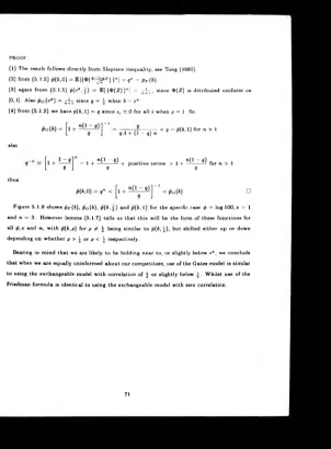
5.1 B idding on a Single C o n t r a c t ...66

5.2 B iddin g on a Sequence o f Contracts ... 73

6. R E C O N C IL IN G TH E F R IE D M A N A N D G A T E S M O D E LS ... 84

6.1 A n Impossibility T h e o re m ...84

6.2 Characterising O rder Independent Distributions ...87

7. TH E T E N D E R E R ’S D E C ISIO N PR O B LE M ... 98

7.1 Formulation o f the P ro b le m ... 98

7.2 A R eview o f the M A B P and its Solution ... 99

7.3 Generalising the M A B P ...105

8. F U R T H E R R E SE A R C H ... 113

A C K N O W L E D G E M E N T S

Research for this thesis was carried ou t whilst I was in receipt o f a Science and Engineering

Research Council Studentship. I must also thank my supervisor Dr. Jim Smith for m any

helpful discussions.

D E C L A R A T I O N

S U M M A R Y

T he problem s faced b y a com pany in determ ining its bids on a sequence o f con tracts put

ou t t o tender has been studied extensively in past literature. T h is thesis concentrates on

formalising and developing these existing m odels as well as presenting new m od els for both

the com peting bidders and the tendering organisation.

Development o f these m odels involves reviewing and extending theoretical results in the areas

1 . I N T R O D U C T I O N

1.1 T h e S e q u e n t ia l B id d in g P r o b le m .

Organisations such as public authorities and large companies are often required to em ploy

outside contractors to carry ou t work for them . T h e usual method o f awarding such a con tract

is to put it out to tender, as follows. The organisation w ill invite a sm all number o f com panies,

from a larger p ool o f com panies, to subm it a b id , o r estim ate, o f th eir charge for the work.

It is com m on for the com pany submitting the low est bid to be autom atically awarded the

contract, especially when the work is o f a m oderate co s t. If the same organisation is sequentially

tendering sim ilar contracts t o the same p ool o f com panies we shall refer to the problem s faced

by the tendering organisation (tenderer) and bid d in g companies (bidders) as The Sequential

Bidding Problem. The aim o f this thesis is t o present m athem atical m odels for both the

tenderer and the bidders to assist in their decision making process in a sequential bidding

environment.

The tenderer’s problem is, for each contract, to select a subset o f th e p o o l o f com panies w ho,

on the one hand, he believes will between them q u o te a low bid, and on the other hand will

provide him with useful information as to which com panies to invite t o b id in the future. W hen

formulated mathematically this leads to a stoch astic control problem w h ich is a generalisation

o f the well known m ulti-arm ed bandit problem.

The bidder’s problem is t o select a bid that is large enough to ensure a reasonable profit,

but small enough to have a significant chance o f w inning. He m ight also take into account

the fact that consistently high bidding may alienate the tenderer and result in him not being

invited to bid on future contracts.

Before discussing the problem further, and ou tlin in g the aims o f this thesis, it is worth

emphasising the appropriateness o f the Bayesian approach for m odelling this problem. M ost

practitioners w ould accept that the role o f a m athem atica l sequential decision m odel is to pro­

vide and update basic parameters that the m odels operator should then use, in conjunction

with any subjective information he may have, t o form ulate a decison a t each time period. A

Bayesian m odel has the attractive feature that it perm its, and indeed encourages, the incorp o­

ration o f subjective inform ation at all time periods. T h is is particularly useful in a sequential

bid d in g environment where subjective information is likely to be readily available. For exam ple

on e m ay learn that a particular bidder is likely to be behaving differently for the next contract

or tw o, fo r, say, financial reasons.

W e now consider the possible approaches to modelling the problem .

A n am bitious way to model the whole problem is to use a gam e theoretic model w ith the

tenderer and the individual bidders as players, i.e. a model w here it is assumed all play­

ers are behaving rationally. An appropriate m odel m ay be based o n the ideas o f Harsanyi

(1 967,1968a,b). T he basic principles underlying such a model are briefly outlined in chapter

8. It should be emphasised that many player games o f this type are immensely com plex, and so, in ord er to make progress, we must look to simplify the problem somewhat.

T h e first step in this simplification is to look at the problem s facing th e tenderer and bidders

separately. As mentioned above, the tenderers problem can be form ulated as a stochastic

co n trol problem - this is the subject o f chapter 7. W ith the p roblem faced by an individual

bid d er w e have two choices o f approach. T he problem can be m odelled in a game theoretic way

w ith ju s t the com peting bidders as players, or alternatively we can lo o k at the problem faced

by an individual bidder in a decision theoretic framework. The d ecision theoretic approach

means w e assume our com petitors are behaving predictably in som e sense, for example drawing

their bid s randomly from some fixed distribution. This approach is th e subject o f chapters 4,

5 and 6.

G a m e theoretic models with ju st the bidders as players have received some attention in the

literature, stemming from the papers o f Griesmer 8 Shubik ( 1967a,b,c). Other contributions have c o m e from Sm ith 8 Case (1975), Engelbrecht-W iggins (1980), H olt (1980) and King

8 M ercer (1988). However the vast m ajority o f the bidding literature is devoted to the decision th eoretic approach to the bidders problem , mostly revolving around the papers o f Friedman

(1956) and Gates (1967). Chapter 3 provides a review o f this m aterial.

Sum m arising, this thesis does not consider any game theoretic m odels. In the main we

con cen tra te on formalising and extending existing decision theoretic m odels for the bidder’s

and ten derer’s problems as well as presenting new models and exam ining related topics. We

shall th u s now develop the basic notation and assumptions for the p roblem .

The first point to note is that in order to eliminate the effects o f the different costs o f different

contracts it is com m on to w ork in terms o f a com panies markup, m, rather than their b id , b.

If we consider ourselves as assisting an individual bidder in determining their bids, then we

define ou r markup as m = b/c, th e ratio o f our bid to our point estim ate o f the cost to us o f

fulfilling the contract, c. We shall define the other bidders markups as the ratio o f their bid to

our point estim ate o f the cost o f th e contract, c, we thus might refer to this as our com petitors

apparent m arkup. It is worth n otin g that this definition o f markup is equivalent to defining a

com petitors markup relative to their own cost and then assuming that ourselves and all our

com petitors are using the same p o in t estimate o f the cost o f the contract.

O ur bid d er’s decision problem is now to select a markup. Our actual bid will then be given

by this m arkup tim es our estim a te o f the cost t o us o f fulfilling the contract. O f course the

true cost w ill be a random variable, C , since at this stage the final cost will be unknown t o us.

T he sim plest criteria on which t o base the selection o f our markup is to maximise immediate

expected profit (m - 1)E [C p (m ) ] where p(m ) is the probability that we win the contract w ith

markup m . This probability is clearly uncertain to us and so, as Bayesians, we must treat it as

a random variable, indexed by m . We now make the assumption that the random variables C

and p (m ) are independent for all values o f m. In practice this means that we are assuming our

com petitors w ill not change their procedure for choosing a markup for contracts o f different

costs. If the sequence o f contracts have similar costs this seems a very reasonable assumption.

W ith this assumption the e x p ected profit can now be written as c ( m - l)p (m ) where c = E [C ]

and p (m ) = E [p(m )]. Thus the p rob lem reduces t o com puting an estimate o f p ( m ) - this is the

starting poin t for most o f the existin g models discussed in chapter 3.

As m entioned above, this thesis mainly concentrates on mathematical models. It is however

intended th a t the models presented are flexible enough to allow some o f the many practical

problem s encountered in a real bid d in g environment to be incorporated. In som e cases this is

actually done, and in others it is indicated how it m ay be done. We thus close this introduction

to the sequential bidding p roblem by mentioning a few o f these practical considerations, the

main references here are Ward 8 Chapm an (1988) and King 8 Mercer (1985).

(i)M ore realistic utilities : In th e discussion above the criteria used to choose a markup

was sim ply maximisation o f e x p ected profit. In reality a bidder may wish to consider other

properties o f a con tract, for exam ple the prestige a ssociated with winning a given contract. Or

he may be happy to take a smaller m arkup for a very co stly contract. One way to overcome

this is to define a utility taking into account the relative im portance o f expected profit and

these other features. O ur markup w ould then be chosen t o maximise this utility. An example

o f such a utility is given in §4.3. If we wish to m odel ou r com petitors as also reacting to

factors such as prestige and cost we must look to build a m odel that can handle these factors

as regressors in the estim ation o f p (m ). A m odel o f this ty p e is discussed in §4.5.

(ii) N on-price fa cto rs : A similar consideration to th e above is that o f non -p rice factors

i.e. factors, other than profit, that w e might wish t o consider when choosing our markup.

A n example o f this is our available resources at the tim e o f each contract. Clearly if we win

a contract and d o not have the available resources t o d o the work we w ill incur a cost in

em ploying further staff or buying m ore equipm ent in ord er to fulfill the contract. So the event

o f us winning the con tract at tim e t, w hich w ill clearly affect our resources at tim e t + 1, will tend to make us bid less com petitively at tim e t + 1 as we w ill need a larger profit to cover any extra costs incurred as a result o f having less resources available. M athem atical formulation

o f this leads to a stochastic control problem - a brief review o f the literature on this is given

in chapter 3.

(iii) Seasona/ effects : Clearly, in m any bidding environm ents, such as building works, factors

such as tempereature and number o f daylight hours are g o in g to affect the num ber o f contracts

available and thus the level o f com p etition for these con tracts. These seasonal effects can easily

b e incorporated into the specification o f p (m ). This is discussed in sections 4.3 and 4.5.

(i\ )C o st estimation : One o f the m ajor problem s w ith attem pting to m odel a com petitors

behaviour is that the variability in their cost estimate can sometimes swam p subtle changes

in their markup policy. Some authors have gone as far as concerning themselves more with

estim ating the cost that a com petitor is likely to com e u p w ith than with their markup, see

for example Naert 8 Weverbergh (1978). In chapter 5 we present a model which attem pts to overcom e this by seperating the variability in cost, and th a t in markup.

(v ) ‘on e o ff’ inform ation about com petitors : It is co m m o n for a bidder to obtain informa­

tion about com petitors other than that found ou t sim ply from their bidding behaviour. For

resources. Inform ation o f this kind is clearly im p ortan t in determ ining a b id as it will affect

a com petitors behaviour. It is thus desirable that m odels have the ability to incorporate this

type o f information. This is discussed in §4.5 in relation to the m odels o f chapter 4.

(v i) The ten d erer’s non-price criteria : Clearly if it is believed that th e tenderer is not

neccessarily going t o award the contract t o the lowest bidder, this w ill have a significant effect

on the estim ation o f p (m ). Ward 8 Chapm an (1988) discuss this p oin t in detail. However for contracts o f a reasonable size and im portance it is very likely that a tenderer would have

sufficient knowledge o f potential bidders t o only invite com panies to b id w h om he was sure

w ould be capable o f fulfilling the contract satisfactorily. If we assume this t o be the case then

there is no reason t o suppose that the tenderer w ould not award the co n tra ct to the lowest

bidder. We shall assume this to be the case throughout the thesis.

1 .2 S c h e m a ta .

This thesis essentially divides into four parts. Chapters 2 and 3 p rov id e background and

review material. Chapters 4 and 5 present tw o types o f decision theoretic m od els for the bidders

problem . Chapter 6 then examines the relationship between these tw o typ es o f model and develops some interesting theoretical asides. Finally chapter 7 looks at th e decision theoretic

approach to the tenderers problem.

One o f the main tools in any sequential decision m odel is likely to be tim e series analysis and

accordingly chapter 2 is devoted to reviewing standard Bayesian tim e series models which are

then used in chapters 4,5 and 7. As mentioned above, chapter 3 provides a review o f existing

decision theoretic m odels for the bidders problem .

T h e first part o f chapter 4, sections 4.1 -4 .3 , form alises on e o f these decision theoretic models,

the Gates m odel, and develops it into a sequential m od el. Section 4.4 develop s a multivariate

analogue to one o f th e time series m odels mentioned in chapter 2 and §4.5 then applies this to

the m odel described earlier in chapter 4 to provide a pow erful sequential version o f the Gates

m odel. Similarly chapter 5 produces a sequential version o f another m odel discussed in chapter

3, the Friedman m odel.

Chapter 6 examines the relationship between the G ates and Friedman m od els and as a result o f this defines and characterises a new class o f finitely additive distributions.

T h e tenderers decision problem is form ulated in chapter 7 and shown to be a generalisation

o f the standard m u lti-arm ed bandit problem (M A B P ). The M A B P is then reviewed and an

attem pt to extend the solution ideas for the M A B P to the more general tenderers problem is

given.

Chapter 8 then addresses som e issues that there has not been tim e to develop in the main part o f the thesis.

Finally it is worth noting that in a thesis such as this which addresses the same basic problem

from a number o f different viewpoints it is essential to get clear in ones mind exactly which

problem is being tackled in each chapter. Thus at the begining o f chapters 4,5,6 and 7 a sort

o f mini introduction is provided to clarify the assumptions used, the problem addressed and

2 . A R E V I E W O F B A Y E S I A N T I M E S E R I E S M O D E L S

2 .1 T h e B a y e s ia n A p p r o a c h t o T im e S e r ie s A n a ly s i s .

The classical A R IM A tim e series m odels o f B ox 8 Jenkins (1970) work on the idea that a series can be m odelled by first detecting and rem oving n on-stationary com ponents, such

as trend and seasonality, and m odelling the resulting stationary series as a sum o f random

variables, which they later assume t o be normal. T w o practical criticisms can be levelled at

these models. Firstly, any attem pt to move away from the normality o f the com ponents in

the model for the stationary series will lead to problem s o f tractability in the m odel fitting.

And secondly, the attem pt to remove all the features o f the series before any modelling takes

place does n ot allow any room for heuristic reasoning in the model building process, which

would be very desirable if the modeller had a g ood knowledge o f a particular series. A further

more general, but related, criticism is that the m od els are to o rigid and d o not easily allow an

operator to incorporate any extra information he m ay receive as the m odel is running.

These problem s led practicioners t o develop an alternative class o f Bayesian tim e series

models. Bather (1965) proposed a class o f n on -n o rm a l state space m odels which he showed

to be fully tractable. A very flexible normal state space m odel, the Dynam ic Linear Model

(D L M ), was introduced by Harrison 8 Stevens (1976) as follows. An observed series {Y t } is related via a linear model to an underlying m arkov series {0, } which has som e heuristic meaning and is consequently known as the state, or level, o f the series. This is summarised in

the equations below,

Observation equation : Yt — F t0t + V, V, ~ W (0 ,V ) (2.1.1)

System equation : 0, = G t0 ,_ , + W , W , ~ Y ( 0 , W ) (2.1.2)

the error com ponents V, and W , are independent, w ith the values o f V and W being prespec­

ified. The v ector F , is a known vector o f regressors as in the ordinary static linear m odel, and

the matrix G , is a known state transition matrix w h ich can be used to m odel factors such as

growth trend and seasonality. The analysis o f the m od el proceeds as follows.

Let D, denote all the data up to and including tim e t, and take the prior distribution

then (2.1.1) and (2.1.2) give

#, |D ,_ , ~ JV(a,,Rf )

t , | D t ~ fV (m ,, C ,)

where the updated values m t, C t are given by the Kalman filter equations, Kalman (1963), as

follows,

a, = G ,m , !

R , = G « C , _ i G ^ + W (2.1.3)

m , = a , 4- s, e ,/(F ,r R ,F , + V )

C , = R , - 8,s,77 ( F ,r R ,F , + V )

w ith st = R ( F t and et = Yt — F ^ a ( . Kalman originally derived these equations for updating

the first tw o cumulants o f $t w ithout distributional assumptions. Harrison 8 Stevens showed that they were also the appropriate equations w ith the state vector and observations being

normal. Harrison 8 Stevens then go on to provide full forecast distributions for {Y t+k | D t-1) . An im portant special case is when F e = G , = I , the identity m atrix , for all t. This is

called the steady model since the evolution on 0t given by (2.1.2) results in its mean remaining unchanged bu t its variance growing at a constant rate. Smith 8 Miller (1 9 8 6 ) develop a non­ normal steady m odel, w ith a multiplicative system equation, similar to on e given by Bather

(1965). T hey then apply this m odel to the prediction o f records.

Am een 8 Harrison (1985) discussed the difficulty o f specifying a value for W . First they noted that the updating from C , _ i —* R , in (2.1.3) simply has the effect o f increasing the

variance com ponents o f C t_ i - They then showed that for the normal D L M the updating given

by

R , = B ( G | C t- i G,r B,

where B , is a diagonal discount m atrix whose elements are all greater than 1, is formally

identical to the updating from C , _ , -♦ R , in (2.1.3). Sm ith (1988) has taken these ideas

further and shown that when G , = I this updating, which he refers to as a spread steady

model, is a sound method for representing dissolution o f information in n on -n orm al models.

This will prove very useful in §2.3.

The DLM overcom es many o f the lim itations o f o f the A R IM A models. The series is modelled

directly which positively encourages input from an inform ed modeller, both in the model

specifications and via intervention when the model is running. Extensions away from the

normality assum ptions are the subject o f the following two sections.

The next section reviews an evolution on the state 0, that is sim ply applicable to all distri­

butions and is in all im portant respects the same as the steady m odel described above. In §2.3

we review the D ynam ic Generalised Linear Model which a ttem pts to generalise the full DLM

to non-norm al distributions.

2 .2 T h e P o w e r S t e a d y M o d e l.

Consider first the steady DLM where 0, is a univariate param eter. The observation equation

(2.1.1) is clearly equivalent to saying

Y, \0t ~ N (0 t , V )

which can easily be generalised to n on-norm al likelihoods for Yt \0t . The cru x o f the model

however is the evolution o f the parameter 0t , that is

t* \ D t —* 0t+\ I D, (2.2.1)

In the steady D LM this is given by the additive equation (2 .1 .2 ) which, w ith a normal dis­

tribution on 0t , presents no problems as normality is preserved under addition. However if

0, is n on-norm al, an additive equation such as (2.1.2) presents problems o f tractability in com puting the distribution o f 0t+ , | D t .

Smith (1979) took the view that rather than state the form o f the evolution (2.2.1) and then

examine its consequences, one should define the properties one wants an evolution to have and

then look for a transform ation on the density o f 0t \Dt that has these properties. Smith chose

to define his desired properties on a decision space associated w ith the parameter 0t as follows,

(1) The Bayes decision, with respect to any step loss fu n ction , on the random variable

0t+i\Dt should be the same as the Bayes decision on the random variable 0t \D,

(2 ) If 0,\Dt has a unim odal density, then the expected loss, w ith a step loss function, o f a

Bayes decision on 0,+ I |D, should be at least as large as the expected loss o f the same

Bayes decision on 0t \ Dt

These properties effectively define what Smith means by a steady evolution on 9t . Smith

then proves that the only transformation on the density o f 9t \Dt to satisfy these properties, as

well as some regularity conditions, is o f the form

/ , + l (*«+ , |D.) a [ / , ( * , | D ,)]k* 0 < fc, < 1 for all t (2.2.1) where f t+ l is the p.d.f. o f tff+1|D, and / , is the p.d.f. o f 9t \Dt . Smith called the process 0, undergoing the evolution (2.2.1) a pow er steady model, and if k, = k for all t he called it a simple pow er steady model. One feature o f the m odel is that, unlike a m odel using a well

defined system equation, it does not provide the join t distribution across {9 t+ i,0 t I D t }- A t

first sight this may appear to be a deficiency o f the model. However Smith & Miller (1986)

and Smith (1988,89a) argue that this is not so, pointing out that the crux is that the m odel

provides well defined forecast distributions across observables.

In practical term s the model is very useful as the evolution (2.2.1) is easily applicable to

non-norm al distributions on 9,. It is also very flexible in that the evolution can be applied to

transformations o f the parameterisation o f 9,, allowing the evolution to be applied to natural

parameterisations. For example in §4.1 the evolution (2.2.1) is applied to a multivariate logistic

transform o f a set o f probabilities.

An interesting property is that, unlike the steady D LM , the evolution (2.2.1) does not

neccesarily im ply that E[0, +1 \ D t\ = E [0, | D t \, it is however always true that m ode [0,+ j | D t] =

m ode [9, \ D t ].

Smith (1981) develops these ideas t o a multivariate parameter T he natural extension is

to take an evolution o f the form

/ , ♦ . ( * « ■ I A ) « [ / , ( * , | D ,)]* 0 < * < 1

which is perfectly valid but has the slightly restrictive im plication that 9 ['] | } undergoes

a simple pow er steady evolution with the same value o f k for each i, 0J' 1 being the i ,h element o f

For situations where it is believed that this sym m etrical development on the elements o f 0t is

inappropriate, Sm ith proposed the stacked steady model as follows. First reorder the elements

quicker than inform ation about 9\ for * = 1 , . . . , n - 1. T h e stacked steady m odel is now

defined by letting 0\ |0J + 1, . . . ,0 " develop w ith a simple pow er steady m odel with discount factor k, for i = 1, . . . , n, where 0 < k, < k, + ! < 1, i = 1, . . . , n - 1.

2 .3 T h e D y n a m i c G e n e r a li s e d L in e a r M o d e l.

In this section w e review the D ynam ic Generalised Linear M odel (D G L M ) as proposed by

West, Harrison © M ig on (1985). T he D G L M attem pts to generalise the full D LM , as defined

by (2.1.1) and (2 .1 .2 ), t o n on-norm al distributions on the observed series and the state. The

price that has to b e paid to make this generalisation work is that the state 0t is m odelled as

a second order process, i.e. only inform ation about its first tw o cumulants is m aintained, and

no distributional assum ptions are made. T h e model does however provide a full distribution

across the observables {V -, } . T he m odel is defined as follows.

In place o f the observation equation (2.1.1) observations are assumed to com e from an

exponential family likelihood as follows,

p {Y , \ r )t A ) oc czp{<t>(ritYt - a ( q , ) ) } (2.3.1)

where % is the natural param eter for Yt . T he system equation is as before i.e.

(2.3.2)

but now the distribu tion o f W , is unspecified. The param eters q, and 0t are connected via

the guide relationship

g(n t ) = F f 0 , (2.3.3)

where g (.) is a know n function, quite possibly g ( x ) = z , and F f is a known vector as in the

DLM.

The priors on rjt_ l and 0,_ i are as follows,

rh - l \Dt. l ^ C P [ c . l , 0 i . l } (2.3.4)

~ ( m - i . C , . » ] (2 3 .5 )

where C P [.,.\ denotes the conjugate prior for the likelihood (2.3.1) which has p.d.f.

p (q ) oc ezp{ar\ - /? a (q )} (2.3.6)

Equation (2.3.5) does not specify a full distribution for 0t ~ i | A - i but sim ply says it has

cumulants given by

E [ # , - » | A - i ] = m , - i

V a r [ # ,_ » ! I V , ] = C , _ ,

The development (2.3.2) on 0 , - i gives

r,, \ D t .t ~ C P [ a ; , ^ ] (2.3.7)

0, | D , _ , ~ [ a , , R , ) (2.3.8)

where

a t = G ,m ( - j (2.3.9)

R, = B , G , C , _ ,G ^ B ,

N ote that the updating from C t_ i —• R , is achieved by using a discount matrix B t , which, as

noted in §2.1, is a perfectly sound m eth od for representing dissolution o f information about 0t in this non-norm al environment.

In order to obtain the values o f , 0', on e can use the guide relation (2.3.3) as follows. Define

/ , = F f a , (2.3.11)

q, = R ,F ,

then from (2.3.7) com pute E[g(r;t ) | D t- i } and Var\g(qt ) \ D t -1] m functions o f ci't ,0't . It is then clear, that by taking the mean and variance o f each side o f (2.3.3) and equating them,

that the following equations can be used to solve for a j , 0\ as functions o f a , , R ( , f t and qt .

V [g (n ,)\ D t- l ) = f , (2.3.12)

V a r i a n t ) I D t-1] = qt

Consider now updating the param eters a't ,0't ,a t and R , in the light o f an observation Yt ,

hence obtaining the updates for the d istribu tion s r)t I D t and 0,\ D t

Substituting these into (2 .3 .1 4 ) gives

*“ » = • « + s ,(g , - f t )/qt (2.3.15)

C , = R , - (8t8,r ) ( l - P,q,)/q,

where g, = E [0(»j( ) | D tJ and pt = V ar[g(t},) | D t] which can be com puted from the full distri­ bution o f tf, I D , given in (2.3.13).

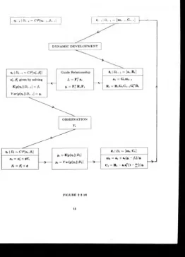
The full scheme o f u p datin g parameters is given in figure 2.3.16.

•h

, I

, ~

i|

FIGURE 2.3.16

2 .4 T h e B e t a - B i n o m i a l D G L M .

In this section we review a specific D G L M , the Beta-B inom ial. T h e reason for this is to

provide a background for sections 4.4 and 4.5 which are devoted to developing and applying a

multivariate analogue to this model.

The model is specified as follows. Observations com e from the likelihood

p(Yt | Mi, n ,) = ( y t) ^ ' ( l “ /**)"'_ r *

= ( y ( ) e i P { y ' lo8 J*~~ ) + n‘ ' ^ i 1 _ M*) } (2.4.1)

which, by com parison w ith the exponential family likelihood (2 .3 .1 ), immediately gives the

natural parameterisation as

If one now takes the guide function, </(.), to be the identity, i.e. g ( x ) = x , then the model is

specified by

fi, = G « * , - ! + W ,

which can be described as a dynam ic version o f the standard log isitic-lin ear regression model.

The conjugate prior for ij, in the likelihood (2.4.1) is the L o g istic-B eta distribution, L B e (a t , 0 t ), w ith p.d.f.

and cumulants

p{Vt I a , , 0 t ) =

r

(

o

<

0t

e

-""

r

(

a

,)

r

(

A

) (

i

+

«”•)“•+<’1

E[»?«] = •?(<*«) - 7 ( A )

V a r ( t i , ) =

7(at) + 7(A)

where 7 is the digam m a function and 7 the trigam m a function defined by

Also one can com pute

mode(rit ) = log

and the curvature o f p(tj, | a t , 0 t ) at the mode as

Qi A <*t + 0t

Refering to figure 2.3.16, assume we have set and hence obtained a t , R , and,

from the guide relationship, f t and qt . The next task is to obtain a', and 0[ by solving

/ , = 7 ( 4 ) - 7( t f ) Qt = + 7 ( # )

this however requires numerical solution. So West et. al., pointing ou t that the guide relation

really is just a guide, suggest, as an approxim ation, taking / , as the mode o f r), \ D t- 1 and qt as the inverse o f the curvature o f p[r)t \ D t - i ) at the m ode. This gives the sim ple form ula

= - ( l + e 'O Qt

« = i ( i + . - ' • )

Moving dow n figure 2.3.16 the updating from to a t ,(3t is given by

a , = a j + Yt

0 , = f i + n, - Y,

Note that this appears slightly inconsistent with figure 2.3.16, this is sim ply due to using the

parameterisation a t ,0 t to make the L ogistic-B eta be in its standard form. T o be consistent

with figure 2.3.16 w e would have to use the parameterisation a , , (a , + 0 t)/

nt-The values for gt and p, are given by

9t = 7(<*«) - 7 (ß t)

Pt = 7(<*,) + 7 (/9.)

All other updating is as in figure 2.3.16.

An interesting special case occurs when G , = I and F , is the same for tw o succesive time

periods. In this case one way o f m odelling a dynam ic developm ent directly on ijt would be to

use the power steady m odel, resulting in th e updating

a't = k ,a t- i

It is easily shown that, in this special case, the B eta-B inom ial D G LM is equivalent to the

pow er steady model with

_ V a r ^ - i l D t - i ) * V a r f o l D , - ! )

F T C t_ 1F " F T B , C « _ , B , F

where F is the com m on value o f F ,_ t and F f .

3 . A R E V I E W O F D E C I S I O N T H E O R E T I C B I D D I N G M O D E L S

As noted in chapter 1 the two main models proposed are due to Friedman (1956) and Gates

(1967). It should be emphasised that both these models were proposed primarily for bidding

on o n e -o ff contracts, and not for sequential bidding.

T he m athematical framework in which both these models exist is as follows. We represent

company, or firm, 0, F0, com peting against com panies Fi t . .. , F „ . A s described in chapter 1

our task is to com pute p (m ), an estimate o f p (m ), where

p (m ) = P (we win the con tract with markup m )

The Friedman and Gates models both propose p (m ) should be expressed as a function o f

P i ( m ) ,. . . ,p n(m ), where p ,(m ) is an estimate o f

P i(m ) = P (w e ‘ beat’ Ft w ith markup m )

precisely what is meant by ‘ beats’ is discussed in a moment. Explicitly, the Friedman model

proposes,

p H = f l P ' N (3 1 )

and the Gates model proposes,

#( m ) - <s 2)

The merits o f these two models have been discussed extensively in the literature, resulting

in a supposed controversy as to which is best to use. Before m entioning som e o f the main

contributions to this controversy it is worth highlighting an unfortunate recurring trait o f

papers in this area. M ost authors feel they have to answer the question “which o f Gates’ or

Friedman’s formulae is right ?” . Surely this is the wrong question t o be asking. Alm ost any

formula can be deemed to be right if we make the appropriate assum ptions. T he questions

should be, firstly - which assumptions vindicate the Friedman form u la and which the Gates

formula ? and, secondly - which o f these assumptions are most likely to be appropriate in our

given situation ? One o f the aims o f §4.1 is to isolate the underlying modelling assumptions

and im plications if the Gates formula is to be valid, so that the practitioner can determine

whether or not it is appropriate to use it. T his poin t has also been made by King © Mercer

(1987,88) w ho attem pt to isolate the assumptions underlying the Friedman and Gates models

from a more practical viewpoint.

A ttem pts t o answer the question o f whether the Friedman or Gates form ula is right, have

been b o th experim ental (i.e. based on perform ance in sim ulation) and theoretical. T heoretical

attem pts t o ‘ p ro v e ’ the Gates form ula right have com e from Rosenshine (1972), w ho also

provides a g o o d review o f the controversy, and D ixie (1974). However Fuerst (1976) has

highlighted errors in both these proofs. Fuerst goes on to make som e interesting points abou t

the G ates form u la, which we mention in a m om ent.

Gates (1976) and Benjamin 8 M eador (1979) have performed sim ulations t o try to ju stify form ula (3.2). T h e Gates sim ulation was sum m arily dismissed b y Fuerst (1977). Benjamin

8 M eadors sim ulation was very similar t o G ates’ and so many o f Fuerst’s criticism s also apply here. T hey also failed to take in to accou n t the com m ents m ade by Fuerst (1976), on w hat

might be a corre ct application o f the Gates m od el. It is worth noting that in all o f these

simulations the Gates model perform ed significantly better than the Friedman model.

Before com m enting further on (3.1) and (3.2) w e define two sets o f random variables. Let X ,

be a random variable representing the bid m ade b y com pany *', * = 1. . . n, o n a given contract. A lso, for a m ark u p m , define the random variable 0, (m ) by

0j(m ) = p(F i wins the contract| we use m arkup m )

We can thus m od el the problem by working w ith either the vector o f bids X = ( X i , . . . X n )

or the vector o f probabilities 8 (m ) = (0o ( m ) , . . . , 0n ( m ) ), that is, in practice, start by putting

a prior o n either o f X or tf(m ). In §4.1 w e show th a t the Gates form ula (3.2) follows directly

from a D irichlet prior on # (m ).

The Friedman form ula (3.1) clearly arises from putting independent priors on X l t . . . , X n

and interpreting P i(m ) as p (c m < X i ) , where c is ou r point estim ate o f the cost o f the contract

to us.

T he above com m ents on the Friedman and G ates m odels lead us to make the following

definitions. A ‘ Friedman type' m odel is one which p u ts a prior directly on the random variable

X . W hilst a ‘ G a tes type’ model is one which puts a prior directly on 0(m ).

Thus chapter 4 presents a sequential G ates typ e m odel, and chapter 5 presents a sequential

Friedman type m odel.

Gates’ ow n justification for his m odel was as follows. Assume that com p an y F, has a, balls

in an urn, and that the con tract is awarded by drawing a ball at random from the urn. Then

p (m ) = * o /5 Z r « o *•» w here *o »■ the number o f balls we have in the urn. If the relar

tionship P i(m ) = *0/(* o + * .) , is assum ed, G ates’ formula follow s by substituting =

* o (l - P i[m ))/ p i(m ), in the form ula fo r p (m ).

This ju stification inspired Fuerst (1976) to make the correct, and indeed obvious, deduction

that if we know the exact distribu tion o f X l t . . . , X n then p ,(m ) should be interpreted as

p , (m ) = P (F 0 beats Ft w ith m arkup m | F0 or F, w in the con tract)

= P (c m < X i | F0 or Fi w in the contract)

Since w ith this interpretation th e G ates form ula is a probabilistic identity. This interpre­

tation o f P i(m ) is also obvious from the form alisation in §4.1. It is however at odds with the

interpretation originally intended b y G ates and used by Gates (1976) and B enjam in 8 Meador (1979) in their simulations. In these they sim ply took P i(m ) = P (c m < X i ) . For fixed m use

o f this interpretation o f p ,(m ) is equivalent to assuming that the event o f F0 beating F, is in­

dependent o f the perform ance o f F0 and Fi relative t o the other bidders. In chapter 6, theorem 6.1.4, it is p roved that, provided P ( X i = X , ) = 0, there is no countably additive distribution

across X , , X , such that for all * in a given range P ( x < X t ) = P ( x < X , \ X i < X } ). We

can thus con clu de that G ates’ form ula is never a probabilistic identity, for all m , with G ates’

original interpretation o f P i(m ).

Decision th eoretic m odels oth er than those o f Friedman and G ates have co m e from , amongst

others, Agnew (1972), Curtis 6 M aines (1974), Attanasi 8 Johnson (1975), G unter 8 Swanson (1978), Carr (1982) and K n od e 8 Swanson (1987). Agnew is one o f the few to specifically tackle the sequential problem . He uses a novel non-param etric approach which starts with

just a point estim ate o f the m axim um o f the profit function (m - l)p (m ). T h is estimate is

then sequentially updated using techniques o f stochastic approxim ation. T h e on ly information

required for th e updating is w hether or n ot we w in each contract.

Curtis 8 M aines and Carr claim t o have broken free from the influence o f the Friedman and Gates m odels by placing m uch m ore em phasis on the variability o f each com petitors cost

estimates. C laim in g, perhaps ju stifiably, that in many cases this variability is more im portant

than variability in markup in accounting for variability in the final bid. However in both these

papers the m e th o d s used to com pu te our probability o f winning rely on the independence o f

com petitors b id s and in principle differ little from the Friedman approach.

T he p apers o f Attanasi 8 Johnson, Gunter 8 Swanson and K node 8 Swanson are repre- sentitive o f a different, and im portan t, approach to the problem . Their main thrust is that

n on-price fa c to r s such as a com petitors resources are at least as im portant as profit in de­

termining a com p etitors bid. T hey thus form ulate a stochastic control m odel to maximise

expected p ro fit u p to some finite horizon, given that when a con tract is won this will affect a

com petitors a b ility to bid com petitively at future tim e periods.

N on -p rice fa c to r s such as resources are discussed in more detail in Ward 8 Chapman (1988) and King 8 M e rcer (1985).

An extensive bibliography containing over 500 references on all aspects o f the bidding prob­

lem has been com p iled by Stark 8 R oth k opf (1979). M ost o f the references however relate to very specific bidding environments such as defence or oil industry contracts, and tend to

recommend v e r y tailor made bidding procedures, relying little on general mathematical models.

U ltim ately it is o f course desirable to incorporate aspects o f o f these tailor made procedures,

as well as n o n -p r ic e considerations, in to the m ore m athem atical models. One o f the features

o f the m od el in chapter 4 is th a t, although prim arily a m athem atical m odel, its framework

does perm it in corporation o f other in form ation. T h is is discussed in sections 4.3 and 4.5.

4 . A S E Q U E N T I A L G A T E S T Y P E M O D E L

In this chapter we assume ourselves t o be assisting an individual bidder in determining his

bids on a sequence o f contracts. T h e basic assum ptions are those outlined in chapter 1, namely

that C II p (m ), and that the tenderer w ill award the contract to the bidder making the lowest

markup.

The model outlined in sections 4.1 t o 4.3 and generalised in sections 4.4 and 4.5 can work

on the assumption that the on ly inform ation our bidder receives after each contract is the

value o f the lowest markup, or b id , m ade by the other bidders. T h e identity o f the winner

when we do not win can be in corp ora ted , but is not needed in updating our estimate o f p (m ).

Other information, such as the id en tity o f the other bidders or the actual values o f their bids,

is n ot used in the m odel as stated. However the m odel could be extended to incorporate such

information. Thus, as it stands, this m odel would be useful in an environm ent where we would

not expect to receive much inform ation in the afterm ath o f a con tract being awarded.

4 .1 A F o r m a lis a tio n o f t h e G a t e s M o d e l .

In the last chapter G ates’ own ju stifica tion for his m odel was described. In this section we

construct distributional assum ptions which lead to G ates’ formula and confirm Fuerst’s obser­

vations about the interpretation o f the probabilities p, (m ). These distributional assumptions

are then shown to lead naturally t o a sequential version o f the G ates m odel. In the next sec­

tion it is shown how this sequential m od el is easily extended to a sim ple power steady m odel

o f the form discussed in chapter 2. In §4.3 ways o f incorporating som e o f problem s faced by

practicioners in to this model are discussed, m ethods for setting prior parameters are given,

and finally there is an illustrative exam ple.

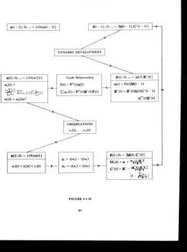
Sections 4.4 and 4.5 show how the m odel can be further extended to a Dynam ic Generalised

Linear M odel, allowing m odelling and on line estim ation o f seasonal and regressor effects.

The first step in our form alisation o f the Gates m odel is to define ou r random variables. For

a given markup m let

tf(m) = ( 0o (m ) t . .. , 0n(m )) is sim ply an unknown param eter vector, and so, as in any Bayesian

analysis, we start by putting a prior distribu tion on it. Since som ebody must w in,

$3"_o 0%(m ) = 1- Thus consider the prior,

(♦ o ( m ) ,i | ( m ) ,... . » „ H - P K H . a . H , . , . , a r (m ) ) (4.1.1)

where P ((a 0(m ), a , ( m ) , . . . , a n (m )) represents the Dirichlet distribution with parameters

a0( m ) , a i ( m ) , . .. ,a „ ( m ) . O f course p (m ) = 0o ( m ) , and the natural estim ate o f 0o (m ) is its expectation, thus take

« " » > = E [»„(m )| = (4.1.2)

2_».=o a '

Suppressing the dependancy on the index m for th e tim e being, we now transform to new

parameters.

Let fa = Oo/{0o + ^i)i then it is easily show n th a t (V>,,1 — fa ) ~ P (a o><Xi), i-e a

Beta distribution (see De G root (1970) ), so E[V»i] = a 0 /(oco + « . ) = f a , say, where fa is an

estim ate o f fa . Therefore, transforming to new param eters fa , ct, = a 0( l — fa )/ fa , substituting

this in to (4.1.2) yields

P M = E (*„] = i l + £ j (4 1 3 )

N otice that fa has the role ofp< in G ates’ formula (3 .2 ). T o interpret f a ( m ) is thus to interpret

P i(m ) in the G ates formula.

Clearly since fa — 0o/(0o + 0<) we have, directly fr o m the definition o f the 0’s,

^ . _ P(F 0 wins contract) p (F0 or Fi wins the con tra ct)

= p{Fo wins the contract | F0 o r F, wins the co n tra ct) (4-1-4)

So as Fuerst(1976) points out, the Gates form ula is valid provided P i(m ) is interpreted as

f a (m ) above. We note this is not the usual interpretation o f p ,(m ). T o obtain these values in

a practical environment, we must ask the question, “ G iv en only us or com pan y « can now w in

the contract, what is the probability that we win ? ” .

We can thus conclude that G ates’ formula is consistent w ith a Dirichlet distribution on 0 (m ).

T he Dirchlet assumption (4.1.1) suggests a way in w h ich the record o f success o f the com p a­

nies F i, . . . , Fn in previous similar contracts can be in corp ora ted to obtain im proved estim ates

o f E[0O]- T o m otivate this process, assume first that we always chose the sam e markup m.

Initially ch oose a 0 ,o i i , ■ ■. , a n so that they are consistent with our beliefs a b o u t p ,(m ). How

this might be done in practice is discussed in §4.3. Now consider the award o f th e contract as a

Bernoulli trial w ith n + 1 types o f success 0 , 1 . . . , n. A type » success o ccu rs w ith probability

0, and is equivalent to com pany F, winning the contract. Thus

So the relevant probabilities can be updated directly once we learn w ho w on th e last contract.

We have n ow established how, for fixed m, we can update the probabilities p (m ) and p ,(m )

when we know the identity o f the winner, F* say, o f the last contract. In order that we

can update these probabilities for all m , suppose we are told that after all the bids had

been subm itted, the lowest markup m ade by our com petitors was m ‘ , and th a t the identity

o f the co m p e tito r using this m arkup was F*. We now know that for all fixed markups m

less than m ' w e would have won the contract, and thus would have the follow in g updating,

a £ (m ) = a0(m ) + 1 and a ‘ (m ) = ati(m) for all t / 0. And for all fixed m arkups m greater than m* we w ould have, o £ (m ) = a * ( m ) + 1 and a * (m ) = a ¿(m ) for all « / k. Suppressing

the index m o n a 0, . . . , a n we therefore have the following updating for ou r probabilities: (4.1.5)

where r, is th e number o f type » successes, or equivalently,

f 1 if com pany i has ( 00 otherwiseotherwise

if com pany x has won

Clearly p (0 | r ) oc p (r | O)p(0) thus from (4.1.1) and (4.1.5)

(#(m) | r) ~ P K ( m ) , a ; ( m ) , . .. ,o;(m )) (4.1.6)

where o* (m ) = a , (m ) + r, , in particular,

and,

m < m"

m > m ‘ (4.1.7)

(4.1.8) [q0 + 1] / [oo + <*i + 1]

m > m ‘

and the full distribution o f 0(m ) can b e updated from

<*o (m ) — a 0(m ) + 1

a ,( m ) = a, (m )

a 0(m ) = a 0(

o<.(m) = a,(m ) m > m ‘

A practical problem arises if we are only told the value o f the winning markup, rather than

m * . Although we can use the u p da tin g in (4.1.7) and (4.1.8) when we d o n ot win the contract,

i f we d o win, with a bid m' 11 say, w e know only that m* > m '11. Clearly updating o f p (m ) is unaffected for m < m 111, otherwise, w e may have to o p t for the overly conservative updating

obtained by setting m* = m*1’ .

It has been shown that if we know the value o f our com petitors’ lowest markup after each

con tract, it is only neccesary to estim ate p ,(m ) at the first time period. From then on p (m )

an d p ,(m ) can be updated directly, given only the m inim al information o f our com petitors

lowest markup and the identity o f th e company making this markup - information which is

ofte n easily accessible.

T o obtain an understanding o f how this model works in the long run, it is helpful to consider

th e behaviour o f p (m ) and p ,(m ) as th e number, N , o f ou r com petitors best markups we have

observed gets large. Let these m arkups be denoted by m \, . . . , m 'N , and assume that none are

equ al, so, without loss o f generality, w e can assume they are ordered i.e. m\ < m j < , . . . , <

m'N Repeated application o f (4.1.7) yields

fo r r = 0 , . . . , N , where w e define = - o o and + , = + o o . As N gets large we have,

i.e. the probability that w e win with a m arkup in the range ( m ’ , m ‘ + , ) , tends to the proportion

o f times we would have w on, if we had used a markup in this range at all tim e periods. This is

a pleasingly sensible result, and fits in w ell with Gates’ original interpretation o f his model. We

also note that var(0o ) ~ r ( N - r)/ N 2( N + 1 ) as N gets large, thus var(0o ) —» 0 as TV —» oo. So m € (ro;>ro; + i )

w e can state the stronger result that the random variable 0o tends to (N - r ) / N , in probability,

as N —* oo. We also find,

P i(m | m ; , . . . ,m % ) ~ N - r

N + R, - r m € (rn‘ ,m ’ + l )

where R, is the num ber o f contracts that com pany « w ou ld have w on, if we had used a markup

in the range ( m ; , m ; + 1 ) at every time period. Thus 5Z "= i f t = r> since N - r contracts would

have been won by us. E xactly analogous results pertain i f som e o f the observed markups are

identical.

O ne suprising feature o f the updating form ula (4.1.7) is th a t p (m ) can be u pdated without

knowing the identity o f our best com petitor on each co n tr a c t so far. Thus, one im plication o f

the Dirichlet m odel is that given no other information a b o u t our com petitors, the sequence

o f their lowest bids o n each contract is sufficient for th e prediction o f p (m ). However, if

as is usual, we e x p e ct to gain information about w h o else has been invited to quote for a

particular contract, then the identities o f those com p etitors m aking winning bids is crucial to

our updated p robability p (m ). For exam ple if we have b een told that we are only com peting

against companies F i t . . . , Fk , k < n, then w e have im p licitly been told that ,F n

cannot win. Thus w hen working with the distribution o f 0o ( m ) , . . . ,0 *(m ) we must condition

on the event Y = {tffc+1(m ) = 0 , . . . ,0 „ ( m ) = 0 ) . From D e G r o o t (1970) we have (0o ( m ) , . . . ,0 k(m ) | Y ) ~ P ( a Z ( m ) , . . . , a ; ( m ) )

where currently # (m ) ~ P (a jJ (m ),... ,a * ( m ) ) . So in p a rticu lar, when we have observed a

num ber o f markups, th e probability that F0 wins is now given by

p (m | Y ) = Qk) + So + s . )

where S, is the total num ber o f contracts w on so far by F ,. T h is illustrates how different types

o f information can be utilised to improve p (m ), as em phasised by Ward 8 Chapm an (1988). 4.2 A Stead y M o d e l Version.

An important practical problem in estim ating probabilities is that the policies o f com peting

this are changes in m anagem ent personnel or m anagement policy, or a co m p a n y diversifying

its interests. Because o f this, a com petitor’s behaviour on more recent con tra cts is often more

relevant for making predictions about its future behaviour than what it did in th e distant past.

In the last model we have implicitly assumed that probabilities Oi(m) are s ta tic , i.e. they do

not change with time. T h is leads, for exam ple, to the unrealistic belief th a t given a large

enough N we can be alm ost certain about ou r chances o f winning with a given m arkup m . We

can m od el the probability 0 (t) steadily changing over time by using the Sim ple Pow er Steady

M odel o f chapter 2. i.e. take

where k € (0,1], and / » ( . ) is the p.d.f o f 0 (t) \ . at tim e t. Note, for convenience w e are now

indexing 0 by tim e, t, although it is still o f course a function o f m. This d evelopm en t means

that individual decisions associated with 0 are unchanged. However any uncertainty associated

with these decisions will increase at each tim e p eriod. O f course i f k = 1 w e h ave the static

case considered previously. For general k it is easily checked that this develop m en t implies

. , . . . . _ f [fca0 + 2 - fc] / [3 - 2 k + k (a 0 + a*)] m < m * ’ ' t + 1 - fc] / [2(1 - k) + rj + Ar(a0 + a*)] m > m ’ T o obtain a better understanding o f how this m odel operates we now look at its behaviour

in the lon g run, when the discount is constant between contracts. For a given m , after T

contracts, the updating in (4.2.3) gives

/.♦ »(•(*+

1

(#(l + l ) | r ( « ) ) ~ P ( *«(«) + ! - * ) (4.2.2)

( 9 (t + 1) I r (t + 1) ) ~ P ( k a ( t ) + r ( t + 1) + 1 - * ) (4.2.3) the analogues o f (4.1.7) and (4.1.8) are,

p {m I m ") = [fcoio + 2 - k] / [1 + (n + 1)(1 - *:) + kJ2?=o a <] m < m ‘ [fca0 + 1 - k] / [1 + (n + 1 )( 1 - *:) + *£ ,"= 0 “ •] m > m ‘ and

where

1 if company i has w on the contract at time t

Therefore as T —► oo

(4.2.4)

and thus

p (m ,T ) = E [ « „ ( r ) ] = M I ) ^ r . o V r o j T - t )

E T - o M T ) l + n + ( l - t ) - ‘

since Yli=o r« ( 0 = 1 f ° r *■ A lso, the m ode o f 0o { T ) , M [0o(T)\, say, is given by

M [» „(T )] = - ( ì - t ) È f r o ( r - » )

So if we let M0 = (1 - Jb) 0 *:‘ ro (7’ “ 0> th en M> can be interpreted as a discounted version o f the true proportion o f tim es we would have w on contracts, if we had used this markup m

at all time periods, recalling that 0o (T ) = 0o (T , m ). Now we can write

Tlim p(m,T) =

+ (1 -

where

1 - k )(n + 1) e [0,1)

l + ( l - * ) ( » + l )

thus p (m ,T ) tends to a weighted average o f the discounted true p roportion and a state o f

complete uncertainly, represented by our probability o f winning being l / ( n + 1). We also note, from (4.2.4), that

(T il -

[ l - t + M „ | [ l + p ( l - t ) - M o l

So, unlike the static case, var{90(T)\ /♦ 0 as T —* oo. Hence we can make n o statements about

the convergence o f the random variable 0O■ We have thus avoided the som ew hat unrealistic

consequence o f the static Dirichlet model o f b ecom ing completely certain abou t our chances

o f winning with a markup m as the number o f past contracts T —» oo.

An alternative form o f the steady model is to apply the evolution in (4.2.1) to a trans­

formation o f 9 (t). In particular we might think o f the multivariate log istic transform given

’’•(

0

=iog(£{o)

i=1

... n

(this is used more extensively in the Dynamic Generalised Linear M odel o f sections 4.4 and

4.5). Applying this steady evolution to if(t) gives

(#(t + l ) | r ( 0 ) ~ P ( * « ( 0 )

and

(»(‘ + 0 I r(l + 1 ) ) ~ r ( t « ( l ) + r ( l + 1))

the analogues o f (4.1.7) and (4.1.8) are,

| _ f [* «o + 1 ] / [ 1 + * E . " = o Q<] p (m |m ) = | (

and

[*a0] / [ l + ’=0 a,]

[*a0 + 1] / [1 + *(a0 + a

[fca0]/[l + fc(a0 + a,)]

i < m" i > m*

. .v / l*a0 + 1] / [1 + k (a Q n >r. ) = |

» < m

i > m* p^(m | m ' ,

Once again look in g at the asym ptotic behaviour, w e have after T contracts

a , p ,) = * ’ - « . (0) + f > ' r . ( r - l ) therefore as T —► oo

and thus

(1 2 4)

p ( m , r ) - = Mo

(1- * ) - *

S o in this case p ( t ,m ) tends to the discounted true proportion. Once again, o f course,

war[ff0(7’ )] / * 0 as T —► oo so we can make no com m ents a b ou t the convergence o f the random variable 0o . This alternative evolution illustrates nicely the flexibility o f the steady model in

allowing us to apply steady evolutions to transform ations o f random variables. The trans­

form ation o f $ to t] is particularly appropriate as m any have argued that it is easier and

m ore natural to w ork in terms o f these log odds rather than probabilities, see for example

Spiegelhalter 8 K n ill-Jon es (1986).

In the above tw o cases we have assumed that the drift in information, m odelled by the

parameter k, is the sam e between contracts. Although this m ay be a reasonable assumption to

make if contracts appear at regular, or approxim ately regular, intervals o f tim e, it is probably

m ore realistic t o relate k to the waiting time between con tracts, with more drift o f information

occuring over longer tim e periods. T he simplest way to d o this is to let

1 - 4 = (1 - A )— (4 2.5)

To

W here r is the tim e interval between the tendering o f the last contract and the tendering o f

this one, and r0 is som e base time period, for exam ple, the average time between contracts. Thus k is now a function o f r, and A is a constant we have t o set. Note that under this scheme,

Finally, consider setting the parameter A. From (4.2.5) we have that A is the value o f k

representing the am ount o f drift in 0 that occu rs in time r0. In the next section we explain

how the param eter d = y^"_ , a , - n can be view ed as the number o f data points we think

our current setting o f a is worth. If after tim e r0 we have observed no data, (4.2.1) tells us

that d will be updated to Ad. So we can set A b y answering the question ‘ after a further time

period r0 , w hat proportion o f its present value w ill our current setting o f a be worth ? ’ . This

proportion w ill be A, and will usually be in the range (.8 ,1 ).

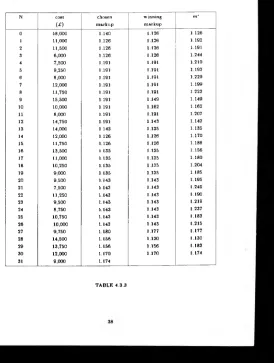
4.3 U sin g T h e M o d el In P ractice.

To use the m odel described in the previous tw o sections we must first set the prior parameters

Q o ( m ) ,... , a n (m ). A t first sight it seems w e m u st specify n + 1 functions o f m , for example

by putting a join t distribution across X t , . . . , X n and setting (m ) from the relationship

O j(m ) = a0( m ) ( l - f a [ m ))/ fa (m ), a 0 (m ) bein g arbitarily specified. However w e can avoid this by con dition in g on the event we do not w in, as follows. Let fa denote the probability that

com pany i w ins the con tract given that we d o n o t. Then it is easily shown that

A plausible m odelling assum ption is that the d istribution o f <fa , . . . , <f>n should not depend on

our chosen markup m. F rom De G root (1970) w e have,

(<t> l . ••• ,<t>n) ~ , a n)

with c * i , . . . ,q„ as in (4 .1 .1 ). So we conclude th a t the parameters , a „ will n ot need to

depend on m either. We also have

E [& ] = fa

If we let P = j then a< = 0 f a . So for a fixed ¡3 we can determine values for , by

estim ating j>,. Clearly represents the p ro portion o f contracts we w ould expect com pany i to

win when we d o not win. If w e are com pletely uninform ed about our com petitors we cou ld set

4>x = l / n fo r all In m ost cases though, we w ill presum ably have som e inform ation about the

past success rates o f our com petitors. This inform ation could be used to fix our estim ate o f fa