A complexity theory of parallel computation

warwick.ac.uk/lib-publications

A Thesis Submitted for the Degree of PhD at the University of Warwick

Permanent WRAP URL:

http://wrap.warwick.ac.uk/112008

Copyright and reuse:

This thesis is made available online and is protected by original copyright.

Please scroll down to view the document itself.

Please refer to the repository record for this item for information to help you to cite it.

Our policy information is available from the repository home page.

A Complexity Theory of

Parallel Computation

Ian P arberry

A dissertation submitted for the degree of

Doctor of Philosophy

University of Warwick

Department of Computer Science

without whose support and encouragement

Chapter 1: Introduction ... 1

Chapter 2: Designing a Parallel Machine Model ... 9

2. 1. The Basic Model ... 10

2.2. The Unit-Cost Measure of Time ... IS 2.3. The Assignment of Programs to Processors ... 18

2.4. Processor Activation ... 22

Chapter 3: Relationships with Other Models ... 27

3.1. A Fixed-Structure Model ... 28

3.2. Shared Memory Machines ... 32

3.3. Reasonableness and Practicality ... 35

3.4. A Practical Model ... 40

3.5. Speedup of Sequential Machines ... 44

Chapter 4: Programming Techniques for Feasible Networks ... 49

4.1. Interconnection Patterns and Programming Tools ... 50

4.2. Recurrent Interconnection Patterns ... 56

4.3. Some Useful Algorithms ... 62

4.4. Reducing the Number of Processors ... 67

Chapter 5: Practical Simulations ... 76

5.1. A General Simulation Theorem ... 77

5.2. A Universal Parallel Machine ... 82

5.3. A Hardware Measure ... 85

5.4. Circuits and Turing Machines ... 96

Chapter 6: High-Arity Machines ... ... 100

6.1. A High-Arity Model ... 101

6.2. The Computational Power of High-Arity Machines ... 103

6.3. A Constant-Degree Universal Machine ... 109

6.4. Examples of High-Arity Algorithms ... 113

Chapter 7: More on Universal Machines ... 120

7.1. Some Lower Bounds ... 120

7.2. A Non-Literal Simulation ... 126

7.3. Oblivious Simulations ... 129

Chapter 8: Conclusion ... 138

Figure 2.4.1 ... 24

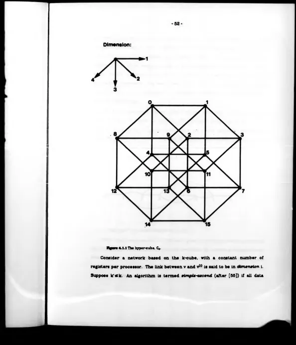
Figure 4.1.1 ... 52

Figure 4.1.2 ... 53

Figure 4.1.3 ... 55

Figure 4.2.1 ... 59

Figure 5.3.1 ... 87

Figure 5.3.2 ... 88

Figure 8.2.1 104

Figure 8.2.2 ... 106

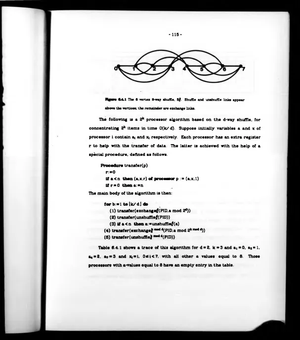
Figure 6.4.1 115

Figure 6.4.2 ... 117

Figure 6.4.3 ... 119

Tables.

Table 4.3.3 66

Table 4.3.4 67

Table 5.1.1 81 Table 5.1.2 81

Parallel complexity theory is currently one of the fastest growing fields of theoretical computer science. This rapid growth has led to a proliferation of parallel machine models and theoretical frameworks. Our aim is to construct a unified theory of parallel computation based on a network model. We claim that the network paradigm is fundamental to the understanding of parallel computa­ tion. and support this claim by providing new and Improved theoretical results, and new approaches to old questions concerning "reasonable" and "practical" models.

This thesis is made up of eight chapters. Chapter 1 contains the introduc­ tion. In chapter 2 we define the basic model, and justify our choice of a unit- cost measure of time, a uniform assignment of programs to processors, and simultaneous processor activation. Chapter 3 compares the network model to a variety of others, including ' fixed-structure networks and shared-memory machines. We explore the concepts of "reasonableness” and "practicality" in parallel machine models, and show that even "reasonable" parallel computers are much taster than sequential ones.

Chapter 1

Introduction

As recently aa I960. Schwartz [62] complained of an apparent lack of theoretical reaulta concerning the computational complexity of parallel or concurrent algorithma.

"In the aerial caae, th e deeign o f algorithms haa com e to be illuminated by a

growing body of th ecretiea l knowledge concerning the ultimate limits o f algorithm

performance.... Until a lik e body of theoretical knowledge has been developed for

highly concurrent algorithms, we will have little basis for judging the extent to

which a given concurrent approach can be im proved."

Two of the most important and fundamental papers in the field of parallel complexity theory (that of Goldschlager [23], later to become [27], and that of Plppenger [S3]) had already appeared by the time Schwartz’s paper reached publication Since then the flow of results has increased from a trickle to a steady stream, and is now threatening to become a flood. Today, parallel complexity theory must be ranked as one of the fastest-growing fields of theoretical computer science.

A theoretical treatment of parallel computation is an attempt to formalize the intuitive concept of a "parallel computer" based on practical experience or reasonable expectations. Amongst the questions which should be addressed by such a formal exposition are the following:

What do we mean by a parallel computation?

What la a good model of a parallel computer?

How should wa design a parallel programming language? Are parallel machines necessarily faster than sequential ones?

What kind of problems can be solved significantly faster by using a parallel algorithm?

Can we obtain asymptotically optimal upper and lower bounds on the parallel resources needed to compute some "natural” functions?

The latter problem appears to be the most popular, judging by sheer volume of contributions (tor some examples, consult [56,73] and the references contained therein). In comparison, relatively little attention has been paid to the first four questions, resulting in a proliferation of parallel machine models in the current literature. Even the most popular model, the shared-memory machine (consisting of a collection of RAMs communicating via a shared memory, see. for example, [20.27]) has many variants. There is a growing tendency to “customize" a machine to allow short, elegant proofs of a particular upper or lower bound, with scant regard to the suitability of the model as a vehicle for further research.

access conflicts (should multiple attempts to write to a shared register be allowed as in [27], or should even multiple reads be disallowed, as in [42]?).

Some of these differences are m erely cosmetic in nature, but some are extremely Important. In order to design a useful parallel machine model, we must first determine which choices matter. We have chosen a model which consists of a network of interconnected RAMs; each RAM can in one step perform an internal computation, or read from or write to a register belonging to one of its neighbours. We believe that the network paradigm is fundamental to the understanding of parallel computation. One attraction is the fact that it possesses a certain theoretical elegance. A RAM is just a network consisting of one processor. A shared-memory machine is just a network where all processors can communicate with a single distinguished processor and no other, and that distinguished processor remains idle throughout the computation. The number of extant papers which use the shared-memory model attest to its ease of programming, and its usefulness as a tool for proving and communicating theoretical results. It is widely accepted, however, that the shared-memory model is not in itself a viable architecture. By placing restrictions on our network model, it is possible to define a practical variant in a far more natural way than is possible with shared-memory machines. This makes the network approach doubly attractive.

The aim of this thesis, then, is to shed some light on the nature of parallel

computation. We shall do this by presenting a unified theory of parallel

computation based on our network model. We shall demonstrate its utility by

providing some fairly eonelse and elegant alternate proofs of results from the

eurrent literature, which will quite often lead to Improved resource bounds or

more general theorems. We will also attempt to provide answers to the

The main body of this thesis Is made up of six chapters. In chapters 2 and 3 we design and justify our parallel machine model. In section Z. 1 we define the basic model, and in section 2.2 discuss the consequences of choosing unit-cost RAMs as opposed to log-cost RAMs as processors. This decision can be summed up by what we call the unit-cost hypothesis: "the unit-cost measure of time is a valid one for parallel processors". We will refer to this hypothesis often throughout the thesis, and conclude that it holds in most situations of Interest. Section 2.3 discusses our assignment of programs to processors, comparing and contrasting it to the S1MD and M1MD approaches of Flynn [19], and section 2.4 our decision to have all processors activated simultaneously at the start of the computation

Chapter 3 compares the basic network machine to a selection of other models. In section 3.1 we propose an alternative fixed-structure variant. It Is shown that a fixed-structure network of 2°(n> processors and a non-recursive interconnection pattern can compute any single-valued Boolean function in a constant number of steps, using an instruction-set consisting of addition, subtraction and logical shifts. In section 3.2 we compare networks to shared- memory machines,and conclude that they are almost identical. In section 3.3 we discuss the possible bounds which need to be placed on the resources of our parallel machines in order to make them "reasonable" or "practical” . The parallel com putation thesis of Goldschlager [27] states that time on a ''reasonable'’ model of parallel computation should be polynomially equivalent to sequential space. Goldschlager places strong restrictions on his SIMDAGs (a variant of the shared-memory model considered in section 3.2) in order to make them obey the parallel computation thesis. We find th at much less strict bounds are sufficient.

our network model, which we call a faaaibla network. This has: (1) Constant degree.

(2) A constant number of registers per processor. (3) An easy-to-compute interconnection pattern. (4) Fixed structure.

We will And later that there is an efficient feasible network which is universal for the general model of section 2.1. Thus the user of such a universal machine has the freedom to program in a high-level language which corresponds to a more powerful architecture at little cost, and the theoretician is provided with a motivation for studying the more abstract models.

Section 3.5 is devoted to exploring the speed-ups which can be made by a parallel machine as opposed to a sequential one. Let B:N-»N be an arbitrary function. Then a T(n) time-bounded deterministic Turing machine can be simulated In tim e 0(T(n)/B (n)) by a network of 20<B*B>*) +T(n) processors. By choosing B (n )* T (n ) we And that every function in NP can be computed in constant time by a network of 2n°(1> processors. Choosing B(n) * T(n)1_* for some c > 0 we And that an arbitrary polynomial speed-up is possible on a machine which obeys the parallel computation thesis. This is a striking result, because an exponential speed-up is not possible for certain natural problems in P unless Pc POLYLOGS PACE.

In chapter 4 we develop the techniques necessary for the construction of

our universal feasible network. Section 4.1 demonstrates the usefulness of the

shuffle-exchange [66] and cube-connected-cycles [55] interconnection patterns.

In section 4.2 we present a recurrent Interconnection pattern CCL* with &

processors and degree 3 with the property that for all k ajkO , CCL* has at lsast

(1) Constant degree.

(2) A constant number of registers per processor. (3 ) An easy-to-compute interconnection pattern. (4) Fixed structure.

We will And later that there is an efficient feasible network which is universal for the general model of section 2.1. Thus the user of such a universal machine has the freedom to program in a high-level language which corresponds to a more powerful architecture at little cost, and the theoretician Is provided with a motivation for studying the more abstract models.

Section 3.5 is devoted to exploring the speed-ups which can be made by a parallel machine as opposed to a sequential one. Let B:N-*N be an arbitrary function. Then a T(n) time-bounded deterministic Turing machine can be simulated in time 0(T(n)/B (n)) by a network of 20<B<,'),)+T(n) processors. By choosing B(n) * T(n) we And that every function in NP can be computed In constant time by a network of 2I>0(>> processors. Choosing B(n) *T(n )'~* for some t > 0 we And that an arbitrary polynomial speed-up is possible on a machine which obeys the parallel computation thesis. This is a striking result, because an exponential speed-up is not possible for certain natural problems In P unless PCPOLYLOGSPACE.

In chapter 4 we develop the techniques necessary for the construction of

our universal feasible network. Section 4.1 demonstrates the usefulness of the

shuffle-exchange [66] and cube-connected-cycles [55] Interconnection patterns.

In section 4.2 we present a recurrent Interconnection pattern CCL* with 2k

processors and degree 3 with the property that for all k *J »0 , CCL* has at least

Meertens [43] we show that any similar interconnection pattern with 2k_1 such disjoint subgraphs cannot share this property. Section 4.3 contains some useful algorithms, and section 4.4 some processor-saving theorems. The latter show that for any machine based on the above interconnection patterns, a P(n) processor network can be simulated on one with F (n ) processors, with a time- loss of 0 (P (n )/ F (n )) for each step. Thus constant multiples in processor- bounds can be ignored without asymptotic time-loss, a fact which simplifies many of our later proofs. A preliminary version of the results of section 4.4 has appeared in [51].

Chapter 5 considers simulations of networks by more practical models. In section 5.1 a general machine-independent simulation theorem is given. Specific instances of this theorem have been seen before in the literature (see, for example. [4.8,21.42,45.71,73]). We use it in section 5.2 to construct our universal feasible network, and again in section 5.3 to simulate networks on width and depth bounded uniform circuits and space and reversal bounded deterministic Turing machines. In section 5.4 we build upon the latter results to improve Pippenger's [S3] simulation of space and reversal bounded Turing machines by width and depth bounded uniform circuits. More specifically, a k- tape Turing machine with space S(n) and reversals R(n) can be simulated by a uniform circuit of width 0(S(n)k) and depth 0(R(n).logaS(n).loglog S(n)). A preliminary version of the work In chapter 5 has appeared In [50].

Chapter 6 generalizes our model to allow high-arlty processors, that is,

processors which have the power to communicate with more than a constant

number of Its neighbours in unit time (and the power to make good use of this

ability). High-arlty machines have appeared in [8,60,70]. Section 6.1 contains

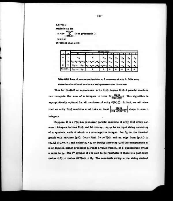
computing power. In particular, a network with arity A(n) and a polynomial number of processors needs time f ) ( , J1. ) to add n numbers, each of

log A(n;

polynomial size, even in the presence of write-conflicts. Thus, for example, a polynomial-processor PRAM with multiple-writes needs time O(log n) to add n polynomial-bit numbers. This is the first lower-bound of this nature to be achieved on a model which allows write-conflicts. Section 6.3 explores simulations of high-arlty machines on constant-degree universal machines of arity 1. As a corollary, we obtain an improved proof of theorem B of [81]. A preliminary version of sections 6.1, 6.8 and 6.3 has appeared in [58]. Section 6.4 contains some examples of high-arity algorithms, most notably the parallel prefix problem.

Section 7.1 is devoted to lower-bounds for universal machines. The universal machine of chapter 5 is found to be optimal for simulations of that nature. The universal machine of chapter 6 is optimal for the simulation of degree-3 machines (Meyer auf der Heide [31] had earlier found it to be optimal for the simulation of constant-degree machines). Section 7.8 contains a new proof of a result of Meyer auf der Heide [33]. In section 7.3 we obtain asymptotic upper and lower bounds o f 0 ( j + log P(n )) for the oblivious simulation of a P(n) processor network on a constant-degree universal machine

with P (n ) processors. This extends the results of Borodin and Hopcroft [8] and

Lang [39], who prove the same lower and tipper bound respectively for

P (n )-P (n ).

It should be noted that this is a theoretical treatment of parallel

computation, and as such Is based upon a number of assumptions which are

widely accepted amongst workers in the field of parallel complexity theory.

the processors are synchronized), we will see in section 3.4 that this is not an important restriction. The advantage of having a synchronous theoretical model is that it is easy to program and reason with. We assume that inter-processor communications can take place within a single instruction-cycle. In the real world, this assumption is unlikely to be true for large numbers of processors; a complexity theory based on this observation will differ quite radically from ours [81], However, we feel fairly safe in making the assumption for networks consisting of a small number (say in the millions) of fairly large processors (about the size of a microprocessor), even though it is unlikely to hold for. say, individual gates in a VLSI chip.

Finally, the reader should note that throughout this work, all logarithms are to base 8, N denotes the set of non-negative Integers. Z the set of integers, and if ceN. deZ. then d mod c is defined to be the unique integer acN such that 0 £ a < c and there exists beZ such that a+bc = d. For those unfamiliar with the "order" notation, we provide the following reminder. Let f,g;N-»R4' (where R* denotes the set of positive real numbers). We say that:

(1) f(n ) = 0 (g (n )) if there exists ceR+, NeN such that for all nfeN, f(n )< c.g (n ). (2) f(n ) = 0 (g (n )) if g(n) * 0(f(n )).

Chapter 2

Designing a Parallel Machine Model

In this chapter we present our basic parallel machine model, and attempt to justify some of the decisions which contributed to its present form. Informally, the model consists of a network of interconnected random-access machines, or RAMs. In the first section we give a more formal description, providing illustration by way of an example RAM instruction-set. We define the major resources of interest; processors (number of RAMs). time (number of Instructions executed), degree (degree of the interconnection pattern), space (number of registers required) and word-siss (the size of those registers). In order to simplify the presentation of algorithms, a high-level pseudo­ programming language is sketched.

The second section is devoted to a discussion of our choice of a unit-cost measure of time. We have chosen to charge a single unit of time for each instruction executed, rather than charge according to some notion of "difficulty". This raises an interesting question: for which instruction-sets is this a valid measure of time? We shall see in subsequent chapters that the answer can be provided in many different ways.

Flnally, In the fourth section we justify our decision to start the computation with all processors active, rather than have them become active at run-time. This latter approach places a not altogether unreasonable upper- bound on the number of processors used in a computation, in relation to time. We shall see in chapter 3 that it is sometimes profitable to consider machines with a larger number of processors. Within this limitation, however, the two models are equivalent.

2.1. The Basic Model

Our parallel machine model can be loosely described as an infinite collection of interconnected -random-access machines, only finitely many of which are active in any particular finite computation. By "random-access machine" we refer to a variant of the RAM. which is already well-known as a sequential machine model (see, for example, [1,12,63]); and by "synchronous" we mean that the instruction-cycles of the RAMs are synchronized. Each RAM has an infinite number of general-purpose registers r0.ri.... each of which is capable of storing a single integer, and a number of read-only registers which are Initialized at the start of a computation. These include the processor identity register PIO and the input-size register SIZE. The PID of the Ith RAM is preset to l, for i ■ 0,1....

More formally, a network M consists of a program and a processor-bound. The program of M is a finite list of instructions; each instruction has the form either:

(ill) Perform an Internal computation. (iv) Conditional transfer of control, or halt.

For example, let denote a binary operation defined on integers. For convenience we divide our example instruction-set into two categories. Local instructions have the form:

goto m if r, > 0 (conditional transfer of control)

Communication instructions have the form: r(«-(rrj of r*) (read) (rr, o f rj)«-!^ (write)

The program is to be executed synchronously in parallel by the (finitely many) active processors. As far as local instructions are concerned, their behaviour is that of independent RAMs, that is. references to registers in local instructions are treated as references to their respective local registers. Execution of a read instruction:

by processor p has the following effect. Suppose registers rj, n, of processor p

contain the values q and p' respectively. Then the contents of register r , of

processor p' are read and placed into register r, of processor p. Similarly,

execution of a write instruction:

by processor p has the following effect. Suppose registers rt, rj of processor p

contain the values q and p‘ respectively. Then the contents of register rii of

processor p are written into register r, of processor p'. ri«-cons tant

r,*-rj~n,

(load register with constant) (binary operation)

(indirect load) (indirect store)

(store read-only register R) (end execution)

r i*-(rr, of rk)

Multlple reads of the same register are allowed. In the case of multiple writes to a single register, we adopt some reasonable convention whereby a single processor succeeds and is allowed to write its value, whilst all others fall. For example (after [27]) the lowest-numbered processor attempting to write succeeds, or (as In chapter 5), the processor which Is attempting to write the smallest value succeeds, with ties being broken In favour of the lowest- numbered processor. A local Instruction must compete with incoming data on the same basis.

Suppose f:Z*-»Z* and xs<xo.X|... x„-i>. where XieZ for 0 * i < n We will say that x has sis• or Isngth n. and write |x| =n. Let m = max|f(x)I and

1*1 ■»

f„:Zn-»Zm denote the restriction of f to n arguments (we adopt the convention that unused output places are filled by zeros). We will variously refer to x as an

input or input string, and each x, as an argum ent or in p u t symbol.

Suppose M is a network with processor-bound P:N-*N. Let p = P(n) A

com putation of M on input x is defined as follows. Place X| into register r|/pj of

processor (i mod p), and set all other general-purpose registers to zero. Set register SIZE of all processors to n. Simultaneously activate processors 0,1....p-1. These synchronously execute the program of M. For 0 « i < m let y, denote the contents of register r|/p| of processor (i mod p) when all processors have finally halted. We say that M computss t it for all n s 0 and inputs x with

|x| « a f»(x ) ■ <y0.yt... y «-i> .

Let T,S,W:N-*N. M Is said to compute within K m i T(n) if for all inputs of size n. all active processors have halted within T(n) steps. For 0 « t£ T (n ), let St(n ) be the maximum (over all Inputs of size n) number of registers of M with non-zero contents after t instructions have been executed. Then M uses space S(n) if S(n) * o«t*^n) 11 hM tuordsiwt W(n) if every value which appears in a register during such a computation has absolute value less than 2w(n) (note that this includes the inputs, outputs and processor Identity registers).

Notes. (1) We have chosen a unit-cost measure of time. This choice will be discussed in more detail in section 2.2.

(2) The space bound is a measure of the number of registers used in a computation It is slightly unusual - the more usual method (see, for example. [1] for the case of a single RAM) is to define space to be the number of registers which are assigned non-zero contents at any point during the computation. Our reasons will become more apparent in chapter S.

(3) The word-size is a measure of the width of (inter- and intra-processor) data paths, and a measure of register size. This can be combined with our unit-cost measure of space to provide an upper-bound on log-cost space.

Consider the example instruction-set given earlier in this section. So far, we have not specified exactly which binary operations can be used for "•*•". In particular we will be Interested in four types of instruction-sets. Each has two- input Boolean functions (defined on single-bit quantities) and the following Integer operations.

(1) The minimal instruction-set allows addition, subtraction, shifts of a single bit, and extraction of the least-significant bit.

(2) In addition, the rwMtricttd a rithm atic instruction-set allows larger shifts and extractions. Suppose rv > 0

ri«-rj mod 2 ~ *

(3) The fu ll arithmmtic instruction-set is the minimal instruction-set plus multiplication, integer division and remaindering.

rtt-rj’ rk

rt«-rj mod r*

(4) The aztwndid arilhm atic instruction-set is the full arithmetic instruction- set plus exponentiation.

ri*-r/k

A number of questions spring to mind. Are these instruction-sets reasonable? Are they powerful enough? Too powerful? Natural? Clearly an unrestricted instruction-set which allows any computable function as a local instruction is too powerful, but what kind of Instruction-set is reasonable? We will return to these questions in the next section.

Instead of writing algorithms in the low-level RAM language, we will follow the common practice of using a high-level language which can easily be translated Into Instructions of this form. We use the usual high-level constructs for flow-of-control, based on sequencing, selection and iteration. Variables of the form (x

at

if y < (y o f prop— or iPID/ 2j) than statement!

•1m statement«

by a network of P (n ) processors causes the 1th processor. 0*ei<P(n). to simultaneously compare its variable y with variable y of processor k/2]. If It finds that the former is less than the latter, then it executes statement^ otherwise it executes statement«. To aid synchronization, we assume that statem ent and statement« are translated into blocks of code containing the same number of instructions, by filling with NO-OPs (such as r0*-r0) as necessary. All of the algorithms in this thesis will maintain synchronization by virtue of this simple arrangement. As a notatlonal convenience we may occasionally use multiple, concurrent and conditional assignments.

2.2. The Unit-Coat Measure of Time

In section 2.1 we defined the running-time of our parallel machines to be the number of instructions executed (synchronously) before all active processors have halted. That is. w e. charge a single unit of time for each instruction executed. This is termed a u n it-cost measure of time. The use of unit-cost charging is a contentious issue. The alternative is log-coat charging, whereby the cost of an instruction is expressed as a function of the size of its arguments, thus tying the time required for a particular computation to its word-size.

thus hardware.

Even for purely sequential machines, the selection of unit-cost measures versus log-cost is of fundamental importance. Inter-simulations between various log-cost models (for example [1], Turing machines and log-cost RAMs) can be achieved with only a polynomial increase in time, whereas no such simulation can be obtained between unit-cost and log-cost models. For example, in time t a unit-cost RAM with multiplication can compute (without input) a value as large as whereas the same machine with log-cost charging can only compute a value as large as 2t+#(l).

From a purely practical standpoint, the choice of charging mechanism depends on the type of computation in question. If the word-size is sufficiently small, then the unit-cost measure is more applicable. Alternatively, if the values being manipulated grow very quickly with input-size, requiring the use of multi­ word Instructions for quite modest input lengths, then the log-cost measure Is preferable. For example, log-cost would more accurately model a small microprocessor, and unit-cost a large mainframe.

measure of time more attractive, since it alone is independent of word-size, and thus hardware.

Even for purely sequential machines, the selection of unit-cost measures versus tog-cost is of fundamental importance. Inter-simulations between various log-cost models (for example [1], Turing machines and log-cost RAMs) can be achieved with only a polynomial increase in time, whereas no such simulation can be obtained between unit-cost and log-cost models. For example, in time t a unit-cost RAM with multiplication can compute (without input) a value as large as 2*1***1’, whereas the same machine with log-cost charging can only compute a value as large as 2t+,(l).

From a purely practical standpoint, the choice of charging mechanism depends on the type of computation in question. If the word-size is sufficiently small, then the unit-cost measure is more applicable. Alternatively, if the values being manipulated grow very quickly with input-size, requiring the use of multi­ word instructions for quite modest input lengths, then the log-cost measure is preferable. For example, log-cost would more accurately model a small microprocessor, and unit-cost a large mainframe.

The parallel analogue of the sequential computation thesis is the so-called "parallel computation thesis" [9.87]. This states that time on all "reasonable” parallel models Is polynomially related. Furthermore, It attempts to characterize parallel computers by relating parallel time to a sequential resource. More precisely, it states that time on a "reasonable" parallel computer Is polynomially equivalent to log-cost sequential (for example, Turing machine) space. This has two Implications. Firstly, a machine which Is too weak to simulate an S(n) space-bounded Turing machine In time S(n)0(t> Is not

pow erful enough, to be called a parallel machine. Secondly, a machine which Is

so strong that a T(n) time-bounded computation cannot be simulated in space T(n)0(l) by a Turing machine is too pow erful to be called parallel. We will be concentrating mainly on the latter aspect of the parallel computation thesis, since networks with an unrestricted Instruction-set are obviously extremely powerful. Henceforth, by "reasonable" we will mean "not too powerful", in the sense that It Is "reasonable" to expect a parallel computer to have only a moderate amount of resources at its disposal.

arithmetic [30] instruction-sets obeys the parallel computation thesis, so is itself as powerful as a parallel machine.

We claim that the unit-cost measure of time is a valid one for parallel processors. We shall call this the w rit-cost hypothesis. It is framed as a hypothesis because it depends upon the way in which the word "valid" is to be interpreted; we will meet several Interpretations in the remainder of this work. Whilst It is intuitively obvious that the unit-cost measure of time is unrealistic for very powerful instruction-sets which allow the computation of infeasible functions in a single step, we may reasonably expect it to be realistic for fairly weak instruction-sets, such as the minimal instruction-set of section 2.1.

This raises a number of interesting side-issues. We are in effect asking when a unit-cost model Is "reasonable". We have seen that restricting the processors to the minimal instruction-set makes our model "reasonable" in the sense that it obeys the parallel computation thesis. But what do we actually mean by "reasonable"? Do models which satisfy the parallel computation thesis successfully formalize the idea of "parallel computers"? What do we really expect from a parallel machine model? These are amongst the issues that we will address in chapter 3.

2.3. The Alignm ent of Programs to Processors

Although every processor of our parallel machine executes the same

program, our model does not fall precisely into the S1MD category of Flynn [19].

This is because the conditional goto Instruction takes action depending on the

value of a local register, the contents of which may vary from processor to

processor. Thus different processors may be at different points in the program

power to a SIMD one. and to a reasonable subset of M1MD models, including that of Galil and Paul [21],

For the sake of discussion, we will call our assignment o f programs to processors a uniform , one. We use the term "uniform" in the sense of Karp and Upton [36], meaning that every machine has a finite description (in our case, the program and processor bound). A MIMD model is non-uniform in the sense that it allows a different program for each processor; thus an Infinite family of finite descriptions (one for each input size) is needed. Some authors (for example [7,14.59]) use the term "uniform" to denote the fact that an external "constructibility" condition has been enforced on a non-uniform model in order to restrict Interest to machines with finite descriptions.

A SIMD machine is a uniform one in which, at any given point in time, all active processors are either executing the same instruction, o r are dormant. Our high-level pseudo-programming language allows the user to write non-SIMD programs; we believe that this keeps the language simple, elegant and flexible (It may be argued that it gives the user the flexibility to get into a lot of trouble, but the same is often said of the goto statement in modern programming languages). Furthermore, it is not really necessary to force the programmer to write SIMD programs, since a uniform machine can be simulated by a SIMD one without asymptotic time-loss, using the same number of processors and degree, with space and word-size Increasing by only a constant.

Suppose M Is a P(n)-processor uniform machine. We will construct a SIMD

machine to simulate M as follows. Processor 1 of the SIMD machine, 0 «l< P (n ),

simulates processor 1 of M. using variables PC. VPC, NPC, PR. A and V, and an

Infinite array R. PC keeps track of the program counter of the simulated

processor, whilst for J*0, R[J] contains the current contents of Its register rj.

(whlch la a constant, independent of n); when PC = VPC the PC01 instruction of the program of M Is simulated. NPC receives the new program counter value, and If the Instruction involves a data-transfer. A and PR receive the address and PID respectively of the register to be updated, and V its new value. At the end of the cycle, the arrays R are updated to reflect the new register contents, using the information in PR. A and V. whilst PC is updated using the contents of NPC. The process is completed at the end of a cycle In which a halt instruction is simulated.

We present the algorithm in the high-level language of section 2.1. A different interpretation is placed on the control constructs however, in order to make them SIMD. The branches of a selection statement (such as if or ease are tried one at a time, with a processor executing a particular branch if its register contents satisfy the entry condition; all other processors remain dormant during that period. This is opposed to the general (non-SIMD) uniform case, in which all processors are free to start their respective branches at the same time, or to enter and leave the construct at different times.

JL»V:*0 PC =V P C *1 while PC > 0 4 »

for VPC * 1 to program length do if VPC = PC then

PR.A.V * comPC01 instruction of M of "^•-constant" PID.i, const ant •'ri^-rj-rii": PID, i. R[j ]~R[ Ic] "r.«-rrj" PlD.i.R[R[j]]

”rn»q":PIDIR[t].R[j]

" r i-r rj of rk" PlD.i.(R[R[j]] of proca - o r R[k]) ” (*>, of rj,-ni":RU].R(l].R[k]

NPC = com PC*11 instruction of M of "halt'O

"goto m if r, > 0 ":lf R[i] >0 then m "others": PC+1

(R[A) o f proceeeor PR) « V PC*NPC

Thus we see that our uniform model is equivalent to a S1MD one Now, a MIMD model allows a different program for each processor Let AN-»N be such that A(i) is a reasonable encoding of a RAM program (say. using the example instruction-set of section 2.1). for ikO. By "reasonable encoding" we mean that a universal RAM should be able to decode this program, using negligible resources, into a format which allows efficient simulation. A MIMD variant of our model is identical to that of section 2.1, except that processor i of a P(n)- processor network has program A(i). 0 * i< P (n ) A is called the processor assignment function

Then clearly there Is a uniform P(n)-processor machine which can simulate M in resources Rj(n)+Rt(n), simply by computing A*, and then having processor l, 0 * i< P (n ) simulate program A(i). Each processor of the uniform machine has an Identical program made up of two parts, a part to compute A*, and a universal RAM.

Thus we see that (provided the resources needed to compute A are kept to a feasible level) a uniform machine can efficiently simulate a MIMD one. This can be summarized as follows: if a MIMD machine is easy to specify, then it can be specified as a uniform machine. Thus a uniform model is equivalent to a useable subset of the MIMD model.

2.4. Processor Activation

In our model as presented so far, all P(n) processors are activated simultaneously at the start of the computation, and begin synchronously executing the first Instruction of the program at time t= l. We call this the

in itia l activation model. An alternative formulation ( (asy activation ) is to

start off with some small number of active processors (for example, just processor 0, or just those which receive input), postponing the activation of the remainder until run-time. This convention has been adopted by Galll and Paul [21] and Savltch [80],

equivalent to the first approach.

Note that this Implies that a T(n) time-bounded machine can have at most n gontn)) (in the case when only input-bearing processors are initially active), or

2°(T(n)) ( ^ the case when processor 0 Is initially active) processors. Our model Is more general than this, and we shall see In section 3.3 that it doss make good sense to talk about T(n) time-bounded machines with ¿ W * 11 processors.

For definiteness, we will assume that: (1) Initially, only processor 0 is activated.

(2) In a computation on an input of size n, processor 0 is initially given the value of P(n) as part of its input.'

(3) If an Inactive processor has a value written into it for the first time in a computation during time-step t. it becomes active and executes the first instruction of the program during time-step t+1. Thereafter, it is indistinguishable from any other active processor. A processor which has halted cannot be reactivated.

Lazy activation Is essentially the same as initial activation, provided P (n )* 2 0(T<,')). Clearly an initial-activation machine can simulate a lazy- actlvatlon one without asymptotic loss In resources, by simply maintaining an activation flag in each processor. Simulation in the other direction is only slightly more difficult. The problem Is to activate P(n) processors and synchronize them so that they begin the execution of the program of M at the same time. If M has P(n) processors and runs in time T(n), we will show that the simulating (lazy) machine runs in tim e 0(T(n)+log P(n)). whilst increasing space and degree by only a constant amount.

shape of a binary tree (aae figure 2.4.1).

F l f m 1.4.1.The binary tree interconnection p attern with 10 verticee.

Each proceaaor has variables C and P. P holds the value of P(n) (we assume that P of processor 0 Is set to P(n) at the start of the computation), and C the number of processors activated so far (we assume that C of processor 0 starts out at 0). The algorithm consists of a single loop. At each Iteration a new level of the tree is activated; C is used to detect termination. Upon exiting the loop, all processors are synchronized, and execution of the program of M can begin.

Processor 1 activates its children at the next level (processors 21+1 and 21+2) using the high-level statements

(C.P) o f prooswor 2 i+ 1 ; ■ C.P (C.P) of processor 21+2 :■ C.P

another delay, this time of fi atepa (where fi la another auitably chosen constant). Note that the values a, fi depend only on the exact form of the RAM Instruction-set, and the ability of the compiler to generate succinct code from high-level statements. In a high-level form, the algorithm is:

Odd-numbered processors wait for a steps Wait for fi steps

C:*2C+1 while C < P do

(C.P) of prooeseor 2i+l := C.P (C.P) of processor 2H-2 : « C.P C:*2C+1

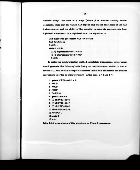
To make the synchronization method completely transparent, this program would generate the following' code (using an instruction-set similar to that of section 2.1, with certain acceptable liberties taken with arithmetic and Boolean expressions in order to ensure brevity). In this case, a = 2 and fi= 1.

1. goto 4 if PIO mod 2 = 0 2. NOOP

3. NOOP *. NOOP 5. C«-2*C+1 6. goto 13i f C * P 7. (C o f 2*PID+ 1)»-C 8. (P of 2*PID+1)«-P 9. (C o f 2*PID+2)«-C 10. (P o f 2*PID+2)«-P 11. C«-Z*C+1 12. g oto 8 13. ate.

¥

2 ___O___ ___ 1____ 3 ____3_____ ___ 3____ H pft p pf p £P9 p GPC p GP f p £PC p £ PC p ft

0 1 7 0 1 4 7 0

2 3 7 0 3 6 7 1 4 7 7 1

3 8 7 1 1 1

6 9 7 1 2 7 1

7 19 7 1 3 7 1 1 |

s ll 7 1 4 7 1 4 7 1

9 12 7 3 3 7 1 3 7 1 10 6 7 3 6 7 3 6 7 3 7 7 ? 7 7 3 7 7 3

12 8 7 3 8 7 3 8 7 3 1 3 1 3

13 9 7 3 9 7 3 9 7 3 2 7 3 2 7 3

. 1 1 19 7 19 7 3 19 7 3 3 7 3 3 3 7 3 1

15 ll 7 3 n 7 3 ll 7 3 4 7 3 4 7 3 4 7 3 4 7 3

16 12 7 7 12 7 7 12 7 7 3 7 3 3 7 3 3 7 3 3 7 3 17 6 7 7 6 .7 7 6 7 7 6 7 7 6 7 7 6 7 7 6 7 7

-ifl 7 7 7 13 7 713 7 7

*-«•»- I A 1 Activation and synchronization o f 7 proceaaora in a lazy-activation

modal. Table e n try show* the value o f the program -counter (PC) and variables P.C

Chapter 3

Relationships with Other Models

The main aim of this chapter ia to compare our network machines to a number of other models. In the first section, we propose a fixed-structure variant of the network model, that is. one in which the interconnection patterns of the machines can be predicted. The more general model computes its own interconnections, which makes it rather difficult to construct as a physical device without increase in degree. It is observed that more efficient machines can be constructed by expending more resources, for example a machine with a non-re cursive interconnection function can compute arbitrary (non-recurslve) single-valued Boolean functions in constant time, given sufficiently many processors.

The second section compares our model to a shared-memory one. In a shared-memory machine, the processors communicate indirectly via a common shared memory, rather than by direct register access. The two models are easily seen to be almost identical in computing power. The third section investigates the concept of a "reasonable" parallel machine touching on such Issues as the parallel computation thesis, bounds on word-size, and restrictions on inter-processor communication.

In the fourth section we define a practical variant of the network machine,

the so-called "feasible network". We expound the desirability of a feasible

network which Is universal for the more general model of section 2.1. Various

types of universal machines are considered, according to the manner In which

they achieve their simulations. In the fifth and final section, we Investigate

possible speedups of sequential machines by parallel ones. Any computable

function can be computed In constant time if sufficiently many processors are

on a muahin» which obeys the parallel computation thesis (and. as we shall see in section 3.3. no such exponential speedup is likely).

3.1. A Fixed-Structure Model

The basic model described in section 2.1 (alls into Cook’s [14] category of machines with "modifiable structure" (since processor interconnections are computed at run-time). This implies that a resource-bound (or such a machine is made up of two parts, corresponding to the resources required to compute the interconnections and those required to perform the actual computation In a "fixed-structure" machine these two components are separated. The former reflects the cost of building the machine, and the latter the cost of using it.

This separation can become significant when the two components differ by a large amount. For example, consider a machine with the example instruction- set of section 2.1, whose only allowable binary operations are (single-bit) two- input Boolean functions, integer division by 2 and multiplication by 2. Let f:(0,lj*-*{0,lj* be defined by f(xo... x„_|)»<yo...yn-i> where fo r 0 « i< n , y( = x, © X(|+i) modn' An coprocessor, constant-degree machine can compute f in a constant number of steps, provided processor i knows the value of (141) modn. 0 < K n , However, the same machine requires (l(log n) steps to actually compute those values. Thus in a model with modifiable structure, the run-time of this machine is O(log n), under a fixed-structure model the run-time is 0(1 ) (and any reasonable fabrication device which Includes addition as part of its instruction- set can compute the Interconnections in parallel in a constant amount of time).

that they can be fabricated aa a completely-connected machine (with each processor connected to every other), but this may involve an unacceptable Increase in degree.

Our fixed-structure model has the same format as the basic model of section 2.1, with a number of minor modifications. Each processor is given a number of additional read-only registers which are preset at the beginning of a computation These correspond to values which are "hard-wired" into the machine during the fabrication process. They consist of the DEGREE register, and an infinite number of port registers Po-Pi.... each of which is capable of holding a single integer.

More formally, a parallel machine consists of a program and an interconnection scheme. The program is a finite list of instructions, each of which may have the following form (where p is a port register). Either:

( 1) Read a value from a register of processor p. (2) Write a value to a register of processor p. (3) Perform an internal computation. (4) Conditional transfer of control, or halt.

In the example instruction-set of section 2.1, the read instruction: r,«-(rrj of nJ

would be interpreted as meaning "read the (rj)th register of processor p^ and place the result into register r|". and the write Instruction:

(fu of rj)«-iìi

would be Interpreted as meaning "write the value from register n, into the (ri)th register of processor p,(".

G:{11 O si < P(n) j x ( d | Owd <D(n) J x N -» {1 1 Owi <P (n ) J.

In a P(n)-processor computation, processor i is connected to processors G(i,d,n). 0 «d < D (n ). We adopt the convention that it ie ( G(j,d,n) | Os: d < D(n) J then je { G(i.d.n) | Ow d <D(n) A com putation of M, where M has Interconnection scheme (P.D.G), is defined similarly to section 2.1, with the following addition. Before the processors are activated, the DEGREE register is set to D(n). and for Owd <D(n), O si <P(n), register p* of processor 1 is set to G(i.d.n). The resources of space and word-size are modified to include the new registers (the word-size of the port registers may be measured according to their absolute contents, or some concise relative encoding, if such is applicable).

Note that a resource bound for computing any given function must Include reference to the complexity of the Interconnection scheme. This is because, as might be expected, more efficient machines can be built by investing more resources in their construction. Information can be stored in the interconnection pattern, to be used later as a kind of "look-up table". Take for example the problem of computing an arbitrary (perhaps non-recurslve) single- valued Boolean function f:(0,lj*-»(0 ,l(. We will show how to compute f on n inputs in a constant number of steps, using n.2" processors.

If x»<X o...Xn-i> is an input of size n, let be a binary encoding of x as an integer. The n.2“ processors are broken up into 2n teams Tt,

0wi<2n. For Owl<2P, team Tj consists of the n processors l.n+J, for Owj<n.

The smallest-numbered processor of each team is a distinguished processor

called the team-leader. For each input x, the team-leader of will have the

value f(x) encoded as part of its interconnection pattern. Our problem then,

given an input x, is to notify the appropriate team-leader.

This Is achieved as follows. Each team-leader sets a specified register a to

the Input to the j0* bit of i. If those two values are different, it writes a one to register a of its team-leader. The team-leader of T ^ , ) will be the only team- leader which is not written to; it then consults its interconnection pattern for the value of f(x), and writes this value to processor 0 for subsequent output.

The following is a high-level implementation of this algorithm. Assume that initially variable x of processor p contains the p1*1 bit (x ,) of the input, 0 * p < n Each processor has two variables i and j which (as in the previous paragraph) record that processor's team number and position within that team. Variable a of the team-leaders will be used for communication with its team members. The result f(x ) will end up in variable r of processor 0.

The interconnection pattern is as follows. For 0 « i < 2 n, 0 < j< n . processor n.i+j (the member of Tt) is connected to processor j (the processor in charge of the j1*1 bit of the input), and processor n.i (its team-leader). For each input x, processor a ln t(x ) is connected to processor f(x ) via a special link. It can determine the value of t(x) by reading the PID of that processor.

a :*r:= 0

i.j: = |piD/ nJ.PID mod n

If (x of processor J) *• 0th bit of i) then (a of processor l*n ):»l if (j * 0 ) and ( a * 0 )

then (r of processor 0) :■ PID of processor special link

Notes. (1) The algorithm as presented uses the extended arithmetic instruction-set. The restricted arithmetic instruction-set can be substituted by increasing the number of processors in each team to 2". If the minimal instruction-set is used, the run-time is 0(log n). Note that the values l.n. 0 * i< 2 ", are not computed at run-time, but are stored as part of the Interconnection pattern.

routing. Information about f(x ) Is encoded using the technique of theorem 4 o f Galll and Paul [21]. The run-time is increased to O(log n) on either the full arithmetic, restricted arithmetic or minimal instruction-sets.

(3) The number of processors can be reduced to 2n*’* [21]. This increases the run-time to 0(n). although it does reduce the degree to a constant, and uses only flnite-state machines as processors.

3.2. Shared Memory Machines

A popular alternative model is obtained by constraining processors to communicate via a common memory, rather than communicating by direct processor-to-processor links. Let D.P,S,T.W,Z:N-»N.

A short d m tm ory mac h in t consists of an infinite number of processors attached to a globally accessible shared memory. Each processor possesses an infinite number of general purpose registers, and a unique read-only processor identity register PID which is preset to i in the 1th processor. ieN. A program fo r this machine consists of a finite list of instructions: each instruction is of the form either:

(l) Read a value from a specified place In the global memory. (li) Write a value to a specified place In the global memory. (ill) Perform an Internal computation.

(tv) Conditional transfer of control, halt.

The allowable internal computations usually consist of direct and indirect

register transfers, logical and arithmetic operations.

More formally, each machine is specified by a program P and a processor

bound P(n). A computation proceeds roughly as follows. An input of sise n

into a unit-size pieces, and the 1th piece is stored in global memory location i. 0 « i < n . All other memory locations and general purpose registers are set to zero. Processors 0.1....P(n)-1 are activated simultaneously; they synchronously execute the program P . When all processors have halted, the output is to be found in some specified place in the global memory.

The processor bound P(n) is a measure of the number of processors used as a function of input size. The space S(n) is the maximum number of non-zero entries in the global memory and registers at any time during the computation. (Note that this includes the input and the processor identity registers). The machine is said to have word-stss W(n) if the maximum value in any register or global memory location during any computation on an input of size n has absolute value less than 2w(n). The time bound T(n) is the number of instructions executed before all processors have halted, again as a function of input size.

Variants of this model have appeared. for example. in [8.14.20.21.27,42,47,62,64.68.69,71.72]. We assume some reasonable protocol for dealing with memory access conflicts, as in those references. The general consensus of opinion is that whilst the shared memory model is a powerful theoretical tool, It is not feasibly buildable using any foreseeable technology.

reference to register r*m of processor 0.

Alternatively, the global m em ory contents can be divided up amongst the processors of the network, provided the instruction-set is sufficiently powerful. Suppose M has P(n) processors and space S(n). Processor i of the network, 0 « i< P (n ). simulates processor i of M. and in addition holds the values of global memory locations i+j.P(n). JkO. A reference to global memory location m is replaced by a reference to register rs.|n/p(B)J of processor m mod P(n) (each processor can reserve its even-numbered registers for memory locations, and the odd-numbered registers for its own use).

This assumes that the instruction-set is at least as powerful as the full arithmetic instruction-set of section 2.1. If the restricted arithmetic instruction-set is used, P(n) should be replaced by 2,l°« I. For a minimal instruction-set, the time-loss is O(log P(n )) per instruction, using P(n) processors. If sufficiently many processors are used (so that each processor holds at most one memory location) this time-loss can be reduced to a constant multiple.

Similarly, a network M can be simulated by a shared-memory machine without asymptotic loss in resources, provided the instruction-set is sufficiently powerful. The registers of the network are stored in the common memory - each processor of the shared-memory machine need only have a constant number of local registers (note that a similar trick serves to reduce the local-memory requirements of all shared-memory machines, subject to similar conditions). A reference to register ri of processor j is replaced by a reference to global m emory location P(n).l+J.

Diis replacement costs only a constant number of steps per access for

machines with the full arithmetic instruotlon-set. As before, if P(n) is replaced

similar result can be obtained by storing, along with each register rt, the contents of r( multiplied by P(n). This requires tim e proportional to

Thereafter, these values can be maintained and used for register access with a constant loss in time for each step of M. Alternatively, the multiplication by P(n) can be computed at access-time, at a cost of 0(log P(n )) per access.

3.3. Reasonableness and Practicality

In section 2.2 we raised the following important question: what constitutes a "reasonable" model of parallel computation? In particular, what is a reasonable instruction-set for our processors, given that we have chosen a unit-cost measure of time? Goldschlager, in [27], placed certain restrictions on his SIMDAG's (a variant of the shared-memory model considered in section 3.2) to ensure that they obey the parallel com putation thesis: time on any "reasonable" parallel model is polynomially equivalent to sequential (log-cost) space. Evidence for this thesis is provided by a multiplicity of "reasonable" models, for example, alternating Turing machines [9], uniform circuits [7] and vector machines [54], as well as Goldschlager's S1MDAG and conglomerate.

The parallel computation thesis also provides us with a powerful theoretical tool. Suppose that we are interested in those problems from P which have an exponential speedup in parallel, that is. those members of P which can be solved in time log0(,)n by a "reasonable" parallel machine. If a "reasonable" machine is one which obeys the parallel computation thesis, then these are precisely the members of P which can be solved in polylog space by a Turing machine.

Let POLYLOGSPACE denote the class of languages which can be accepted in space log0(l,n by a Turing machine. It is widely conjectured that

PC POLYLOGSPACE (although it is not known for sure whether either class

contains the other). Evidence is provided for this conjecture by the existence of

log space complete problems (see, for example. [24.25,26.28.34.35.37]); that is.

problems which are members of P. yet if any one of them is a member of POLYLOGSPACE then PcPOLYLOGSPACE. Thus log-space complete problems probably do not have an exponential speedup on any "reasonable" parallel machine, where the parallel computation thesis is used as a criterion for "reasonableness".

Thus we see that there are two facets to the concept of "reasonableness", that which is reasonable from a practical point of view, and that which is reasonable from the theoretical point of view. It may be theoretically interesting to consider networks with an exponential number of processors (as in section 3.4), but it is certainly not reasonable to consider them as a practical proposition for all except the smallest values of n. A theoretical model is an attempt to capture the essence of an Intuitive notion of "parallel computation"; a practical model is, in addition, governed by physical and technological constraints.

thesis. What exactly are these conditions? Firstly, an S(n) space-bounded nondeterministic Turing machine can be simulated by a network with the minimal instruction-set. In time and word-size 0(S(n)). using the techniques of theorem 2.1 of Goldschlager [27]. Conversely, we have:

Theorem 3.3.1 A T(n) time-bounded network M with word-size W(n) can be simu­

lated by a deterministic Turing machine using space T(n).W(n)+S(n), where S(n) is the space required for the Turing machine to simulate a single instruction of a processor of M.

Proof. Similar to theorem 2.2 of [27], □

This enables us to throw some light on the unit-cost hypothesis. As far as the parallel computation thesis is concerned, it is reasonable to charge a single unit of tim e for instructions which can be computed by a Turing machine in space T(n )0(l^ where T(n) is the number of steps in the intended computation. Given this condition, networks obey the parallel computation thesis provided W(n) * T(n )0(,). Note that this allows machines with as many as 2T(n)0<0 processors; although those who support lazy activation (see section 2.4) insist that P(n ) ■ 2°fr(n)\ and some authors insist that P(n ) = n°*l> (for example, [16,17.42,53]).

To summarize, here are a number of restrictions on network and shared- memory models which can be used to define so-called "reasonable" machines.

(₁) Rastrlcthan* on thm instruction-sat.

Restrictions on Instruction-set are motivated by a desire to see that the

unit-cost hypothesis holds.

(a) The first premise Is that individual processors should behave like log-

be polynomi&lly related to time on an accepted log-coat sequential machine model, such as the deterministic Turing machine (c.f. the sequential computation thesis, section 2.2). Thus instructions which are valid for a T(n) unit-cost-time bounded computation should individually take no more than Tin)0**1 steps on a deterministic Turing machine.

(b) Instructions should be computable in space T(n )0(1) by a Turing machine. This helps to ensure that the parallel computation thesis holds. Note that this condition is implied by part (a ) above.

(2) Bounds upon processors and tim e.

Upper-bounds on the number of processors are usually motivated by the observation that, given enough processors, every computable function can be computed in constant time (see section 3.5), which makes time a singularly uninteresting resource.

(a) P (n )* 2 0fr(n)). This is a consequence of the lazy-activation approach (see section 2.4).

(b) P(n) =n0(1), T(n) = log0(1)n. Machines with these two properties are sometimes called sm all and fa st respectively. See, for example. [16,17,53,59].

(3) Bounds upon w ordsiss.

[27]) by restricting the instruction-set and the size of the input- symbols.

(b) W(n) = T(n)0(,V This condition guarantees that the parallel computation thesis holds, subject to the additional conditions on the instruction-set mentioned in 1 (b) above.

(c) W(n) = n0(1). This ensures that the input encoding is "concise" in the sense of [22]. If the input symbols are allowed to be Integers with more than a polynomial number of bits, then n is no longer a reliable (to within a polynomial) measure of input-size.

Other restrictions are often made in the literature, motivated, it Is often claimed, by practical considerations. These include the following:

(1) Restrictions on degree. It is widely accepted that a completely-connected machine is impractical. Some authors (for example, Galil and Paul [21]) think that degree should be constant (i.e. independent of input-size).

(2) Restrictions on the interconnection pattern In the case of fixed-structure networks (see section 3.1) it is desirable to restrict oneself to machines with an Interconnection pattern which is in a sense easy to compute (see. for example, [21]). This is also the case for uniform circuits [59] and conglomerates [27]. One advantage of this approach is that it avoids the kind of machine described in section 3.1, which can compute a large class of functions (which may even be non-recursive) in an unnaturally small amount of time.

(3) Restrictions on register access. Even if higher-degree machines are

acceptable, should every processor necessarily have the freedom of being

able to read any register of Its neighbours? An alternative is to provide