FOR LINEAR MULTIVARIABLE SYSTEMS
A thesis
presented for the degree of
Doctor of Philosophy in Electrical Engineering in the
University of Canterbury, Christchurch, New Zealand.
by
SAN SHING.CHOI B.E. (H0NS.) ~
12
ABSTRACT
The control of linear multivariable systems (LMS)
where only some of the state variables are directly measurable is considered. The control configurations adopted employ feedback from the measurable state
variables, i.e., the system outputs, via multivariable dynamic compensators. The design problem of determining the compensator parameters is approached via the following methods:
(1) The minimization of quadratic performance indices in the state and control variables, i.e., the optimal control method.
(2) The positioning of the closed-loop system
poles, i. e., the pole placement (or modal control) method. (3) The realization of appropriate state feedback laws through the use of observers.
The optimal output feedback control of essentially noise-free LMS is first examined. A gradient-type solution algorithm is developed that appears to be more efficient computationally than previous techniques; a modified algorithm for handling open-loop unstable LMS is also described. The treatment is then generalized to include cases where the LMS contains appreciable amounts of process and measurement noise; both stationary and non-stationary stochastic problems are considered.
To this end, unres cted-rank pole placement techniques are developed which enable the closed-loop poles to be
positioned t~er arbitrarily close to specified locations, or within prescribed regions of the complex plane. Unlike previous work, new techniques enable exact pole
lacement to be achieved with dynamic compensators having the lowest possible order. Consideration is then given to the more general problems of achieving exact (or approximate) pole placement while minimizing
(a) quadratic performance indices in the state and control variables,
(b) po sensitivi s to small or large system parameter variations, and
(c) steady-state following errors due to measurable and unmeasurable disturbances.
Finally, the construction of minimal-order observers is formulated as a static optimizatiori problem for which a gradient-type solution technique is proposed. The
suitability of using such observers to realize state
TABLE OF CONTENTS
ABSTRACT
ACKNmvLE DGE.HENTS
GLOSSARY
LIST OF FIGURES
CHAPTER 1
1.1
1 .2
INTRODUCTION
EARLY DEVELOPMENTS IN CONTROL ENGINEERING
1. 1. 1 1 • 1 .2
1 • 1 .3
Clas cal trial-and-error techniques
Analytical design techniques
Direct synthesis method of Guillemin and Truxal
LINEAR MULTIVARIABLE CONTROL SYSTEM DESIGN
1.2.1 Non-interactive design technique
1.2.2 Inverse Nyquist array method
1.2.3 Optimal control approach
1.2.4 Pole placement approach
1.3 THESIS ORGANISATION
1.4 PUBLICATIONS
REFERENCES
CHAPTER 2 DESIGN OF TIME-INVARIANT DETERMINISTIC
OUTPUT FEEDBACK CONTROL SYSTKMS USING QUADRATIC PERFORMANCE INDICES
2.1 INTRODUCTION
2.2 OPTIMAL OUTPUT FEEDBACK PROBLEM 2. 2. 1
2.2.2
2.2.3
2.2.4
2.2.5
Problem formulation
Canonical forms for P and N
Main results
Solution algorithms
2.2.4.1 Indirect type
2.2.4.2 Direct type
Numerical example
2.3 OPTIMAL OUTPUT FEEDBACK CONTROLS FOR UNSTABLE PLANTS
2.3.1 Development 2.3 2 The algorithm 2.3.3 Numerical example 2.4 CONCLUSION
APPENDIX A REFERENCES
CHAPTER 3 DESIGN OF OUTPUT FEEDBACK CONTROLLERS FOR STATIONARY AND NON-STATIONARY STOCHASTIC
Page 44 46 47 49 50 51
SYSTEMS USING QUADRATIC PERFORMANCE INDICES 54
3.1 INTRODUCTION 54
3.2 STATIONARY STOCHASTIC REGULATOR PROBLEM 57
3.2.1 Problem formulation 57
3.2.2 Solution technique 63
3.3 NON-STATIONARY STOCHASTIC REGULATOR PROBLEM 64 3.3. 1
3.3.2 3.3.3 3.3.4 3.3.5 3.3.6
The problem
Solution technique
Discussion on problem singularity
Derivation of expressions for gradients Solution algorithm
Suboptimal compensators
64 67 69 71 72 73 .3.3.6.1 General formulation ·73 3.3.6.2 Piecewise - constant gains 74 3.3.6.3 Algorithm for
piecewise-constant gains 76
3.3.7 Numerical example 3.4 CONCLUS ION
REFERENCES
CHAPTER 4 POLE PLACEMENT IN LINEAR MULTIVARIABLE SYSTEMS USING DYNAMIC OUTPUT FEEDBACK 4.1 INTRODUCTION
4.2 POLE PLACEMENT PROBLEM 4.2.1 Problem formulation
4.2.2 Minimum compensator order for exact pole placement
4.2.2.1 Number of independent parameters
4.2.2.2 A lower bound on compensator order
4.2.3 Solution technique
4.2.3.1 Computation the vector h
Page 96 97 4.2.3.2 Computation of the matrix N 98 4.2.4 Algorithm to determine the
minimal-order compensator 99
4.2 5 Numerical example 100
4.3 OTHER POSSIBLE DESIGN OBJECTIVES 101
4.3.1 Pole placement with minimum quadratic performance index 4.3.2 Example
4. 4 POLE PLACEMENT IN PRESCRI'BED REGIONS OF THE COMPLEX PLANE
4.4.1 Problem formulation 4.4.2 Solution technique
4.4.3 The algorithm
4.4.4 Numerical examples 4.5 CONCLUSIONS
APPENDIX A APPENDIX B REFERENCES
CHAPTER 5 POLE PLACEMENT IN OUTPUT FEEDBACK
CONTROL SYSTEMS FOR MINIMUM SENSITIVITY
102 105 107 108 110 112 11 4
117 119 120 122
TO PLANT PARAMETER VARIATIONS 125
5.1 INTRODUCTION 125
5.2 DESIGN TECHNIQUE FOR SMALL
PARAMETER VARIATIONS - PROBLEM A 127
5.2. 1 The system 127
5.2.2 Pole placement problem and the sensitivity function 5.2.3 Statement of Problem A 5.2.4 Algorithm for the solution
of Problem A
5.2.4.1 Solution technique'
5.2.4.2 Computation of the h
127
130
130 130 132 5.2.4.3' Computation of the matrix N 134
5.2.4.4 Solution algorithm 135
5.2.5 Numerical example 5.3 DESIGN TECHNIQUE FOR LARGE
PARAMETER VARIATIONS ...: PROBLEM B 5.3 1 Formulation of Problem B
136
138
5.4
Solution Problem B 5.3.2
5.3.3
.
Illustrative example CONCLUSIONSREFERENCES
CHAPTER 6 DESIGN OF SERVOMECHANISMS SUBJECT TO
Page 140 140 142 144
CONSTANT OR TIME-VARYING RANDOM DISTURBANCES 145
6.1 INTRODUCTION 145
6.2 SERVOMECHANISM WITH UNMEASURABLE
CONSTANT INPUTS 148
6.2. 1 6.2.2 6.2.3 6.2.4
The system
Steady-state error measure System transient performance Analysis
6.2.4.1 Evaluation of dJSS/dK 6.2.4.2 Evaluation of dJts/dK
148 150 151 153 153 154 6.2.5 Possible design objectives 154 6.2.6 Design of dynamic compensator for
simultaneous exact placement
and zero steady-state error 156
602.7 Numerical examples 160
6.3 SERVOMECHANISM WITH MEASURABLE CONSTANT INPUTS
6.3.1 Prbblem form~lation
6.3.2 Analysis
163 163 164 6.4 A SERVOJ.l.1ECHANISM DESIGN PROCEDURE 165 6.5 SERVOMECHANISM WITH STATIONARY RANDOM INPUTS 166
6.5.1 The problem 6.5.2 Analysis
6.5.3 Numerical example 6.6 CONCLUSION
REFERENCES
CHAPTER 7 DESIGN OF MINIMAL-ORDER OBSERVER-COMPENSATORS 167 169 172 172 175
FOR LINEAR MULTIVARIABLE SYSTEMS 177
7.1 INTRODUCTION 177
7.2 THE OBSERVER DESIGN PROBLEM 181 7.2 1
7.2.2 7.2.3
Problem statement Preliminary results
Geometric i tation of condition (ii)
7.3 SOLUTION OF MINIMAL-ORDER STABLE OBSERVER PROBLEM
Page
·186
7.3.1 Canonical form for D 186
7.3.2 Formulation as an
optimization problem 187
7.3.3 Evaluation of gradients 188 7.3.4 Lower bound on stable observer order 189 7 3.5 A design algo thm
7.3.6 Examples
7.4 SOLUTION OF MINIMAL-ORDER FIXED-POLE OBSERVER PROBLEM
7.5 THE OBSERVER AS A DYNAMIC COMPENSATOR 7.5.1 Implementation optimal
state feedback law 7.5.2 Pole placement 7.5.3 Decoupling 7.6 CONCLUSION
REFERENCES CHAPTER 8 CONCLUSION
8.1 CONTRIBUTIONS MADE IN THIS THESIS
8.1.1 Optimal output dback oach
8.1.2 Pole placement approach
8.1.3 Observer-compensator approach
8.2 . POSSIBLE AREAS FOR FURTHER RESEARCH REFERENCES
ACKNOWLEDGEMENTS
I am especially grateful to my supervisor, Dr H.R. Sirisena, for his guidance and constant encouragement. His assistance over the duration of this project has been invaluable.
I am also very grateful to my parents for their most generous financial as stance which made possible my stay in Canterbury, and to my cousin, Miss K.E. Pang, her patience and encouragement.
GLOSSARY
and Definitions
Unless otherwise specified, symbo given below.
have the meanings
II xlf
Ixl
XIJ
I n
0
m,n
X >
X <
X ;::,
/J.
E{x}
.§
wrt
o
(t) 00
0
A i (X)
p[X] = rank [Xl tr{X}
Re{x} Im{x}
n x(t)£R
norm of X modulus of x
transpose of X direct sum
square root of -1, j2
=
-1the n x n identity matrix the m x n null matrix
matrix X is positive definite matrix X is negative definite matrix X is non-negative
is defined as
expected value of x section
with respect to the delta function
definite·
the ith eigenvalue of matrix X
rank of X
the trace of X
the real part of x
the imaginary part of x
RHP LHP RHS LHS LMS MIMO MISO
if and only if implies
is implied by
Right half of complex plane Left half of complex plane Right hand side
Left hand side
Linear multivariable system MUlti-input multi-output MUlti-input single-output
SIMO Single-input multi-output
det determinant
adj(X) adjoint of X
dim (x) dimension of x
col[x1,x 2 ,···xm] columns of x1,x2' · · .,xm max(x
1,x2, . . . ,xm): the maximum value contained ln the set x 1 ' x 2 ' • . • , xm
min(x
FIGURE
1 • 1
1.2 1 .3 2. 1 2.2 3. 1 3.2 4. 1 4.2 4.3
6 . 1
6.2
6.3
7 • 1
7.2
7.3
7.4
LIST OF FIGURES
A general multivariable control system A typical inverse N~quist array plot T~e complete control system
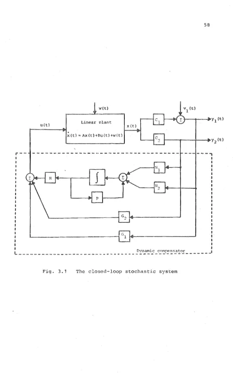
The closed-loop linear multivariable system The linear multivariable control tern The closed-loop stochastic system
Optimal profiles P(t) and H(t)
compensator parameters
Linear multivariable control system
The closed-loop linear multivariable system An arbitrary function of h(cr,w) in
the complex plane s
Linear multivariable servomechanism with unmeasurable constant input w . u
Servomechanism configuration achieving zero steady-state error and exact pole placement
Multivariable system configuration Control of linear multivariable system using Luenberger observer
Reduced-order observer to estimate linear function of state
Asymptotic estimate of Fx.(t) using reduced-ord~r observer Observer as dynamic compensator
INTRODUCTION
1.1 EARLY DEVELOPMENTS IN CONTROL ENGINEERING
Feedback control systems have n in existence for thousands of years. However, until comparatively recently, such systems were not designed formally but were rather the product of mechanical ingenuity. One of the earliest
attempts at analysis was by Maxwell [1] who studied the phenomenon of hunting (instability) in flyball governors. About the same period, Routh discovered his famous stability criterion and by the end of the 19th century, several basic concepts in control engineering, e.g. control loop,
feedback, controller w{th dynamic elements, etc. had begun to emerge [15].
1.1~1 Classical trial-and-erior techn
on the feedback amplifier to the analysis and design of servomechanisms in the frequency (w-) domain, while Bode
[5], MacCol1 [6] and others similarly adapted the results of Bode on minimum phase electrical networks. A second approach to control system analysis.and design is via
Laplace transforms. This so called s-domain approach was pioneered ·by Gardner and Barnes [7] and culminated in the root-Iocus-method (RLM) introduced by Evans [8] about 1948.
The conventional w-domain and s-domaintechniques have one thing in common in that a trial-and-error design procedure is involved. The design process begins .with an educated guess as to the form of a suitable controller whose parameters are tentatively chosen on the basis of a partial analysis. If the complete analysis that follows shows that the performance of the control system does not meet specifications, then the design is modified in a manner governed largely by the designer's experience and intuition.
Th~s is again followed by a performance analysis. The
process is repeated until the specifications are satisfied. The design tools available to the designer are either
graphical or analytical, e.g. Root Loci, Nyquist and Bode plots.
1.1.2 Analytical design techniques
In contrast to the trial-and-error approach,
,
alternative design procedures, called analytical design techniques, have been explored since the early 1940's. Early work in this area included that by Weiner, Hall [3], Bode and Shannon [9], James, Nichols and Phillips [10]
beyond the trial-and-error stage because the methods proceed directly from the problem specifications to the design
without the need human intuition. The design procedure begins with a suitably specified performance index which gives a qualitative measure for the performance the system, Unlike the trial-and-error approach, no licit statement concerning the degree of stability is red
that all solutions must result in the system being Ie and the controller being realizable. The effects of noise on system rformance were also considered. An
excellent text which describes se techniques [ 11] .
1.1.3 Direct is method of Guillemin and Truxal ---~---~--~---Another t synthesis method is that due to Guillemin and Truxal [12]. The design procedure begins with a reduction of the design ifications to a desired closed-loop trans function ch.aracter i zed by its
zerO configuration. A compensator is then designed where the unwanted plant poles zeros are simply
cancelled out. However, specifying the desirable closed-loop transfer function often over-defines the sign
problem, placing unnecessary and undesirable restrictions upon the designer. Furthermore, pole-zero cancellation without regard to internal state variables could result in the system being uncontrollable and unobservable [13].
The trial-and-error, the analytical and the direct synthesis design techniques described above have been developed mainly towards the control of single-input,
this so called classical contY'ol theory was quite well
developed. It was therefore natural to expect that the next of the control theory evolution v.,rould be in the area of multi-input, mUlti-output (MIMO) control system design. Indeed, attempts to solve the MIMO control
problem had been reported as early as 1938 in a paper by Voznesen i [42]"
1.2 LINEAR MULTIVARIABLE CONTROL SYSTEM DESIGN
A fundamental characteristic of mul variable systems is the coupling or interaction between the input and output variables, in that one input af cts more than one output. A consequence of such interaction often is a reduction in the stability margins operation [16]. Hence, the possibility of designing a succession of feedback loops one at a time using well-established classical
feedback theory for a general MIMO system is unlikely to be successful.
To overcome this problem, i t has n proposed that the MIMO system be first decoupled into a number of SISO subsystems by appropriate compensation. This is discussed in the next section.
1.2.1 Non-interactive design technique
Consider the general multivar system shown in Fig. 1.1 with an equal number of inputs in u(s) and
outputs in y(s).
[image:16.566.42.528.28.568.2]u(s) E
!to
F iq. 1. 1
"
Series controller
. K (s)
.
Plant
G(s)
Feedback controller
F (s)
A qeneral multivariable control svstem
When this occurs, non-interaction is said to have been
achieved. Clearly, this results in the MIMO system being decoupled into a system of several S~ISO systems. Then, the classical design techniques mentioned in §1.1 may be used to determine an appropriate diagonal matrix F(s) so that the resulting closed-loop system has the desired performance characteristics. This completes the design procedure.
It was claimed [42] that the non-interacting problem posed above was first solved by the Russian researcher
Voznesenskii in 1938. However, the·first reported work in English was that by Boksenbom and Hood [17] in 1949 where a non-interacting jet engine was synthesized. Subsequent applications of this technique to other practical control problems can be found elsewhere, e.g. [18], [19].
Boksenbom and Hood have approached the problem via a frequency domain technique. Recently, the problem has been considered using state-space (time-domain) formulation
(see e.g. [20]) which in a form more convenient for programming on a digital computer. Although some
contributions in this area have been made by the author and his pro.ject supervisor (see the paper by Sirisena and Choi [21]), the details of this work have not been included in this thesis because i t is felt that non-interactive
design technique is likely to be of limited applicability for reasona listed in Table I.
Advantage'
(A1) Conceptually
Disadvantages
(D1) Complicated controller is usually required to achieve exact
non-interaction [16], [22].
(D2) Excessive of design freedom
is used to make G )K(s) diagonal
leaving little freedom for
improving performance [16].
(D3) If det ~(s)] has RHP zeros, then the resulting design gives unstable or poor control [22].
Table I
[24] where only "approximate" non-interaction is aimed for. The technique is described in the next section.
1.2.2 Inverse method
Consider the LMS depicted in F 1.1. Denote O(s) [G(S)K(S)]-1 and the 1 , J element of 6(s}
"-by q .. (s) •
1J
"
Assume that Q(s}. is of dimension m xm. In the INA method, K(s) is chosen using an
"-interactive and ive process such that Q(s) is diagonal dominant, i.e.
Iq··
11 (s)I
» mE
I
q ..
(s)I
1J
=
d. 1 (s) i 1 I • • • ' , m1
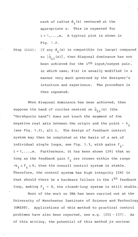
Diagonal dominance may be attained the following steps are followed [24]: initialize design procedure by guessing the form and values of K(s}, then
Step (i):
J,-tep(ii) :
Plot i (s), i
=
1, ... ,m for a range of values of s j w.On locus q .. (s), construct a set of circles
[image:19.566.50.518.49.822.2]each of radius d. (s) centered at the
1
appropriate s. This is repeated for
i
=
1 , •.• ,m. A typical plot is shown inFig. 1.2.
Step (iii): If any d. (s) is compatible (or large) compared
1
to I~
..
(s)I,
then diagonal dominance has not11
.
been achieved for the ith input/output pair,
in which case, K(s) is usually modified in a
manner very much governed by the designer's
intuition and experience. The procedure is
then repeated.
When diagonal dominance has been achieved, then
suppose the band of circles centred on
q ..
(s) (the11
"Gershgorin band") does not touch the segment of the
negative real axis between the origin and the point - k.
1
(see Fig. 1.2), all i. The design of feedback control
system may then be completed on the basis of a set, of
individual single loops, see Fig. 1.3, with gains f.,
1
i
=
1, . . . ,m. Furthermore, i t has been shown [24] that solong as the feedback ga1n f. are chosen within the range
1
-k. ~ f . .( 0, then the overall control system is stable.
1 1
Therefore, the control system has nigh integrity [24] in
that should there be a hardware failure in the ith feedback
loop, making f.
=
0, the closed-loop system is s t i l l stable.1
Most of the work on INA has been carried out at the
University of Manchester Institute of Science and Technology
(UMIST). Applications of this method to practical control
problems have also been reported usee e. g. [25] - [27]. As
[image:20.566.40.521.0.822.2]A
q .. (s)
I I
u (s)
m
1 • 2 A typical inverse Nyquist array plot
1----1----. Y I (S)
G(s) K(s) (s)
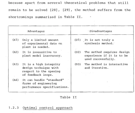
because apart from several theoretical problems that still remain to be solved [28}, [29] I the method suffers from the
shortcomings summarized in Table II.
Advantages
(A1) Only a limited amount of experimental data on plant is needed.
. Disadvantages
(01) , I t is not truly a synthesis method."
(A2) It is insensitive to plant model inaccuracy.
(02) The method requires design experience if i t is to be used successfully.
(A3) I t is a high integrity design techniqu~ with respect to the opening of feedback loops.
(03) The method is interactive and iterative.
(A4) It can handle "standard" forms of engineering
performance specifications.
Table II
1.2.3 Optimal control approach
It is perhaps in recognition of the d~sadvantages
listed in Table I that prompted researchers to abandon the aim of achieving perfect non-interaction. It was also felt
[23] that in view of the reason (D2) given in the same table, the performance of coupled LMS'may be made superior to that of deccmpled LMS.Towards this end/ one of the most powerful design techniques that has been developed to date deals with the design of the optimal feedback system for" a
linear, possibly time-varying plant with quadratic
perfo~ance index [30] . The" pioneering work in this area was done by Kalman [31]. Several texts have since been
written on this particular control topic, see ego [32] [ 34] .
[image:22.566.54.535.49.799.2] [image:22.566.54.527.68.462.2]linear optimal control problem is formulated as follows. Given the LMS
x(t) = A(t)x(t) + B(t)u(t) ( 1 -1 )
X(t)ERn, U(t)ERm are the state and control vectors
respectively. A(o) and B(o) are matrices of appropriate dimensions.
The design objective is to minimize a performance index J(u) whexe
T
J(u) =!x' (T)Sx(T)
+tfo
Xl (t)Q(t)x(t) +u' (t)R(t)u(t)dt (1-2)with the assumption that Q(t) ~o, R(t) > 0 and S).
o.
T is the terminal time. (1-2) is a generalization of the classical integral-square error performance criterion [11].
The solution of the problem is well known and can be derived via Hamilton-Jacobi-Bellman theory. It can be shown that the optimal control u*(t) which minimizes (1-2) exists, is unique and is given by the equation
u* (t)
=
R-1 (t)B' (t)K(t)x*(t) (1-3 )where K (t)
=
K' (t) ). 0 is the solution of the matrix Riccati equationK(t) = - K(t)A(t) -A' (t)K(t) + K(t)B(t)R-1 (t)B' (t)K(t) -Q(t) (1-4 )
with boundary condition
K (T)
=
S (1-5 )The derivation of these results is omitted but can be found
If (1-1) is time-invariant and Q,R are constant matrices, S
=
0 and' T -+00,
the optimal feedback law isn,n
linear and time-inva~iant [31], i.e.
u* (t) == (1-6 )
1\
where
:K
I K > 0 is the solution of the algebraic Riccatiequation
o
( 1-7)The properties of the time-invariant optimal clo loop system described above have also been
investigated, see e.g. [32]. By considering the Nyquist plot of the optimal closed-loop system, i t has been
established that the gain-margin of the closed-loop system is theoretically infinite, while the phase margin is at
o
least 60 [32]. Of course, no physical system can have infinite g n margin due to such parasitic effects as stray capacitance, time delay, 'etc. However, even if the linear models are only approximate representations of the
systems, the gain margin of the optimal closed-loop system may still be very good. The effects of non-linearities and time-delays in the optimal closed-loop systems have also been studied [32].
The design teChniques uS'ing the state feedback laws (1-3) or, (1-6) have since been applied to practical sign problems. For a survey on this, see e.g. [30].
It must remembered that in the formulation of the linear optimal control problem, i t is assumed that the plant is described exactly by' (1 1) and that all the state
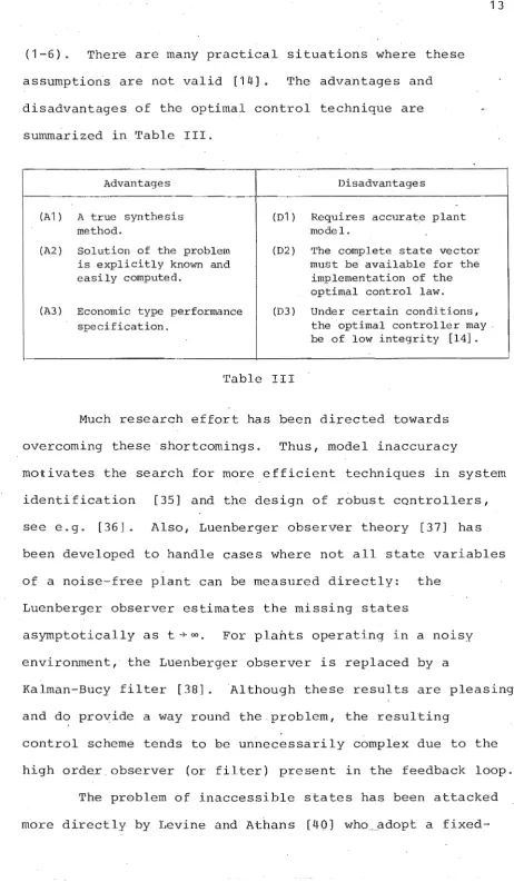
(1-6). There are many practical situations where these assumptions are not valid [14]. The advahtages and disadvantages of the optimal control technique are summarized in Table III.
Advantages Disadvantages
-(A1) A true synthesis (D1 ) Requires accurate plant
method. model.
(A2) Solution of the problem (D2) The complete state vector
is explicitly known and must be available for the
easily computed. implementation of the
optimal control law.
(A3) Economic type performance (D3) Under certain conditions,
specification. the optimal controller may
be of low integrity [14] •
Table III
Much research effort has been directed towards overcoming these ·shortcomings. Thus, model inaccuracy
motivates the search for more efficient techniques in system identification [35] and the design of robust cQntrollers, see e.g. [36]. Also, Luenberger observer theory [37] has been developed to handle cases where not all state variables of a noise free plant can be measured directly: the
Luenberger observer estimates the missing states
asymptotically as t -+ 00. For plants operating in a noi
environment, the Luenberger observer is replaced by a
Kalman-Bucy filter [38] . Although these results are pleasing and do provide a way round the problem, the resulting
control scheme tends to De unnecessarily complex due to the high order observer (or filter) present in the feedback loop.
[image:25.566.65.528.27.822.2]configuration approach with feedback from the measurable states in what amounts to a generalization of classical analytical design techniques [11]. Subsequent extensions
o~ this approach (see Chapters 2 and 3 of this thesis) provide a means for avoiding the use ~f high-order observers or filters.
1 2.4 Pole placement approach
Another synthesis method for time-invariant LMS that has captured much recent research interest is the so called pole placement (or modal control) approach.
Consider now the time-invariant linear system
.
x(t)
=
Ax(t)+
Bu(t), x (0) (1 -8)x(t)ERn, u(t)ERm and the general state feedback law
u(t)
=
Fx(t)Therefore the closed-loop system is given by
.
x (t) = (A
+
BF) x (t)and the solution of the differential equation is
X(s)
=
adj(sI-A-BF) Xo(s) \sI-A-BFI(1-9 )
(1-10)
(1-11)
then the pole placement problem may be stated simplY as: find an appropriate F such that the n roots (A) of the characteristic polynomial IAI-A-BF\ 0, i.e. the poles of the closed-loop system (1-10), assumed some arbitrary
preassigned values.
the po are shifted to desirable positions of complex plane. A common method us.ed is the RLM which is in fact a graphical means of plotting the pole positjonsas a function of f. However, the process can become extremely tedious when involves more than one parameter. There , there is a to develop alternative techniques for handling po lacement problems. Indeed, there has been much. research activity in this area during the last years.
The solution of the pole placement problem posed above is guaranteed to exist provided the plant (1-8) is controllable [39]. For situations where not all the state variables are available, an observer may be constructed to estimate the inaccessible states. However, the same
criticism made ear 1n §1.2.3 concerning the observer order also applies in this case. A more practical approach to the pole placement problem is to use feedback from those state variables which are directly measurable. Several design ,techniques to do this are'currently available 1n the literature, see e« g. [41]. However, un the
technique developed in Chapter 4, they do not, in general, result in the minimal-order controller being obtained.
The pole placement problem is also seen to be, in part, a generalization of the direct synthesis method of Guillemin and Truxal (GT) described in §1.1.3 to MIMO systems. Unlike the GT techn~que, however, the pole placement problem places no restriction on the numerator of the transfer matrix The extra degrees of design freedom obtained as a result may be used to attain other design
1.3 THESIS ORGANISATION
This thesis is devoted to the design of linear
multivariable control systems using the modern state-space approach. Topics investigated include the optimal control terministic and stochastic systems, the po placement problem, the servomechanism problem and the design of
reduced-order observers. Research efforts are directed, in particular, towards developing efficient computational techniques which can be conveniently programmed on a digital computer. All expressions used in the computational
s are also derived.
Perhaps most importantly, i t will be seen that all the techniques described in this thesis employ feedback from only the
measurable state variables> i.e. the plant outputs. TherefoY'e,
difficulty in measuring or estimating the missing state
variables contY'ol purposes neVeY' arises. Also, the controllers cons re .. are usually of lower order than that of Luenberger observers (for the deterministic case) or
Kalman-Bucy filters (for the stochastic case). Then, very much in the spirit of optimal control, the available design
are made use of to obtain the "best" system performance. The degree of "goodness" is, of course, de d on the basis of the design specifications.
Chapter 2 begins with an investigation into the
I
optimal control of essentially noise-f~ee time-invariant systems using fixed-configuration compensators. The maln contribution in this chapter is the development of a
proposed method avoids the solution of non- near matrix equations while appearing to exhibit rapid convergence. Con tion is also given-to the optimal control of open loop unstable plants for which a modified grad algorithm is proposed,
type
The results are then extended, 1n Chapter 3, to the optimal control of linear systems having significant
measurement and process noise. For the stationary and non-stationary stochastic problems considered in this chapter, i t will be shown that the cost and gradients with re to the compensator parameters are not unlike those obtained for the deterministic problem considered in Chapter 2. Therefore, a gradient-tYpe algorithm similar to that scribed in Chapter 2 may be used to obtain the optimal compensator.
From § 1.2.4, i t is seen that .H\Other possible synthesis method is via the techniqu~ of po placement. Thus, in Chapter 4, a new (unrestricted-rank) pole placement technique is presented. It is shown how the pole placement
prob~em can be formulated as a static optimization problem. technique is computationally supc~rior when compared to sting methods and always enables exact pole placement to be achieved with a minimal-order compensator. Consideration is also given to the more general problem of achieving exact or approximate pole placement whi minimizing a quadratic per rmance index in the state and control variables. This is achieved by combining the results obtained for exact pole placement with that contained in §2,2.
only of secondary importance; i t may suffice to position them within a prescribed region of the complex plane. Moreover, this less stringent design requirement on closed-loop poles may be satisfied with compensators of lower order than that required for exact pole placement. Motivated by these reasons, an algorithm to achieve this design aim is developed in §4.4.
In Chapter 5, the sensitivity of closed-loop poles to plant parameter variations is investigated. Two cases are considered. The first case is concerned with situations where the parameter variations are small compared to the nominal values of the plant parameters. A suitable measure of the pole sensitivity is defined and i t is shown how exact pole placement can be achieved at the nominal values of the parameters while minimizing the sensitivity measure. The second case deals with the situations where the parameter variations are not necessarily small compared to their nominal values. An alternative design algorithm based on a new measure of pole sensitivity is then proposed.
In Chapter 6, . the pole placement technique of
Chapter 4 is extended to the design of dynamic compensators for servomechanisms having measurable and unmeasurable
compensator is constructed V1a a function minimization procedure such that optimal transient and steady-state performances are obtained. It is then shown, in the
second step of the design procedure, how the steady-state error due to the .measurable constant inputs can be made' exactly zero through the use of a feedforward controller. The conditions under which such a dynamic compensator
feedforward controller exists are included in this chapter. Consideration is also given to the case where the inputs are actually time-varying Markov processes. The
performance of the servomechanism is assessed by a quadratic criterion. It is then shown that the design problem is
actually mathematically equivalent to the stationary stochastic regulator problem considered in Chapter 3. Therefore, the gradient-type solution algorithm can also be used to obtain the optimal compensator ameters.
Chapter 7 deals with the construction of minimal-order observers. By means of ge6metr arguments, the
observer design problem is reduced to a static optimization problem in certain observer parameters. A systematic
procedure for designing minimal-order stable observers 1S proposed that is based on a new lower bound on the required observer order, a special canonical form for the observer matrix that ensures any prescribed.degree of stability and
a gradient-type function minimization algorithm. A modifie<;i procedure for designing minimal-order observers having
itrarily cified po s is also described. Finally, the role of observers in implementi'ng state feedback l,aws for pole placement, decoupling or minimizing quadrat
In Chapter 8, contributions made in this sis are summarized. Sever areas for future research are also included.
1.4 PUBLICATIONS
Some of the works described in this thesis also appear in the following publications:
CHOI, S.S. and SIRIS~NA, H.R., "Computation of optimal
output feedback gains for linear multivariab systems," IEEE Trans. Automat. Contr., vol. AC 19, pp.257-258, June 1974.
SIRISENA, H.R. and CHOI, S.S., "Design of optimal
constrained dynamic compensators ·for linear stationary stochastic servomechanisms," Int. J. Contr., vol. 20, pp. 363 368, Sept. 1974.
SIRISENA, H.R. and CHOI, S.S., "Optimal pole placement in linear multivariable systems using dynamic output
feedback," Int. J. Contr., vol. 21, pp.661-671, April 1975.
SIRISENA, H.R. and CHOI, 5.5., "Pole placement in output feedback control systems for minimum sensitivity to plant parameter v~riations," Int. J. Contr., vol. 22, pp.129-140, July 1975.
SIRISENA, H.R. and CHOI, 5.5., "Pole placement in prescribed regions of complex plane using output feedback,"
IEEE Trans. Automat. Contr., vol. AC-20, pp.810-812, Dec. 1975.
SIRISENA, H.R. and CHOI, 5.5., "Design of optimal constr'ained dynamic compensators, for nonstationary
linear stochastic system~," Int. J. Contr., to appear. SIRISENA, H.R. and CHOI, 5.5., "An algorithm
constructing minimal-order observers for linear func ons of the state," Int. J. System Science, accepted for
CHOI, S S. and SIRISENA, H.R., "Computation of optimal output feedback controls for unstable linear
REFERENCES
[1] Maxwell, J.C., "On governors," Proc., Roy. Soc. (London), vol. 16, pp.270-283, 1868.
[2] Harris, H., "The analysis and design of servo-mechanism," OSRD Report, 454, Dec. 1941.
[3] Hall, A.C., Analysis and Synthesis of Linear
'Servomechanism, Technology Press, Cambridge, 1943. [4] Nyquist" H., "Regeneration theory," Bell System
Tech. J., voL 11, pp.126 147,'1932.
[5] Bode, H.W., IIFeedback amplifier design," Bell System Tech. J., vol. 19, pp.421 454, 1940.
[6] MacColl, L.A., IIFundamental Theory of Servomechanism," D. Van Nostrand Company, N.Y., 1945.
[7] Gardner, M.F. and Barnes, J.L., Transients in Linear Systems, John Wiley
&
Sons, N.Y., vol. 1, 1942.[8] 'Evans, W.R. ,"Graphical analysis of control systems,1I Trans. AlEE, Appl. Ind., vol. 67, pp.547-551, 1948. [9] Bode, H.W. and Shannon, C.I;:., IIA simplif:i,ed deriva,tion
of linear least square and prediction 'theory," Proc. I.R.E., voL 38, pp.417-424, 1950.
[10] James, H.M., Nichols, N.B. and Phillips, R.S.,
"Theory of Servomechanisms," McGraw-Hill Book Company, N.Y., 1947.
[11] Newton, G.C., Gould, L.A. and Kaiser, J.F., Analytical Design of Linear Feedback Controls, John Wiley & Sons, Inc., N.Y., 1957.
[12] Truxal, J.G., Control System Synthesis, McGraw-Hill, New York, 1955.
[13] Gilbert, E.G., IIControllability and observability in multivariable control systems," J. SIAM Control
[14] Rosenbrock, H.H. and McMorran, P.D., "Good, bad or optimal?" IEEE Trans. Automat. Contr., vol. AC 16, pp 552-554, Dec. 1971.
[15] Fuller, A.T., "The early development of control theory. I,ll University of Cambridge report, CUED/F-CAMS/TR119 (1976) .
[16] MacFarlane, A.G.J., "A survey of some recent results in linear multivariable feedback theory," Automatica, vol. 8, pp.455-492, 1972.
[17] Boksenbom, A.S. and Hood, R., "General algebraic method applied to control analysis of complex engine types,1I Report NCA-TR-980, NACA, Washington D.C., 1949.
[18] Chatterjee, H. K., IIMul tivariable process control," Proc. IFAC, Moscow, 1960, Butterworths, 1961.
[19] Ergin, E.I. and Ling, C., "Development of a non-interacting controller for boilers," Proc. IFAC, Moscow, 1960, Butterworths, 1961.
[20] Gilbert, E.G., "The decoupling of multivariable
systems by state feedback," J. SIAM Control, Vol. 7, pp . 50 - 63 , 1 969 .
[21] Sirisena, H.R. and Choi, S.S., "Minimal-order compensators for decoupling and arbitrary pole
placement in linear multivariable systems," Int. J. Contr., to appear.
[22] Rosenbrock, H.H., "On the design of linear
multi-variable control systems," Proc. 3rd Congress of IFAC, London, 1966.
[23] Mesarovic, M.D., "Control of multivariable systems," Proc. IFAC, MOSCOw" 1960, Butterworths, 1961.
[24] Rosenbrock, H.H., "Design
of
multivariable controlsystems using the inverse Nyquist array," Proc~ I.E.E., vol. 116, pp.1929-1936, Nov. 1969.
[26] Munro, N., "Design of controllers for open-loop unstable mult~variable systems using inverse Nyquist array," Proc. I.E.E., vol. 119,
pp.1377~1382; 1972.
[27] Hawkins, D.J., ,lIPseudodiagonalization and the inverse Nyqui st array method," Proc. I. E. E., vol. 119,
pp.337-342, March 1972.
[28] Rosenbrock, H. H., "Progres s in the design of multi"ariable control systems," Measurement and Control, vol. 4, pp.9-11, 1971.
[29] Rosenbrock, H.H., Computer- ded Control System Design, Academic Press, London, 1974.
[301 Athans, M., "The status of optimal control theory and applications for deterministic systems," IEEE Trans. Automat. Contr., vol. AC-11, pp.580-596, July 1966. [31] Kalman, R.E., "Contributions to the theory of optimal
control," Bol. Soc. 'Mat.Mex., Second Series, vol. 5, pp.102-119, 1960.
[32] Anderson, B.D.O. and Moore, J.B., Linear Optimal
Control, Prent -Hall, Englewood Cliffs, N.J., 1971. [33] Athans, M. and Falb, P.L., bptimal Control,
McGraw Hill, New York, 1966.
[34] Kwakernaak, H. and Sivan, R., Linear Optimal Control Systems, Wiley-Interscience, N.Y., 1972.
[35] Special Issue on System'Identi cation and Time-series Analysis, IEEE Trans. Automat. Contr., vol. AC-19,
Dec. 1974.
[36] Davison, E. J. and Golde'nberg, A." "Robust control of a general servomechanism problem: the servo
compensator," Automatica, vol. 11, pp.461-471, 1975. [37] Luenberger, D.G., "Observers for multivariable
[38] Kalman, R.E. and Bucy, R.S., "New results in linear filtering and prediction theory," Trans. ASME. J. Basic Eng., vol. 83D, pp.95-108, 1961.
[39] Wonham, W.M., liOn pole assignment in mUlti-input controllable linear systems," IEEE Trans. Automat. Control, vol. AC-12, pp.660-665, Dec. 1967.
[40] Levine, W.S. and Athans, M., "On the determination the optimal constant output feedback gains for linear multivariable systems," IEEE Trans. Automat. Contr., vol. AC-15, pp.44-48, Feb. 1970.
[41] Brasch, F.M. and Pearson, J.B., "Pole placement using dynamic compensators,1I IEEE Trans. Automat. Contr., vol. AC-15, pp.34-43, Feb. 1970.
CHAPTER 2
DESIGN OF TIME-INVARIANT DETERMINISTIC OUTPUT FEEDBACK CONTROL SYSTEMS USING PERFORMANCE INDICES
2.1 INTRODUCTION
As pointed out in Chapter 1, one approach to the sign of deterministic LMS is via optimization with re to a quadr c performance index. It is well known that this the unconstrained optimal control involves
om all the state variables and this is, in , impracticable because
(i) opt~mal state feedback law may be unnecessarily compiic Simpler controllers could be constructed for which the overall system performance is still within design specif ations. Such occurrences are quite common, for i t is well known that an optimally designed system tends to have excess gain and phase margins, see e.g. [1] and [2],
(ii) not 1 states can be measured directly. One possibil is to estimate the missing states, using a Luenberger observer [29J. However, the resulting , controller may s 11 be of unnecessarily high order~
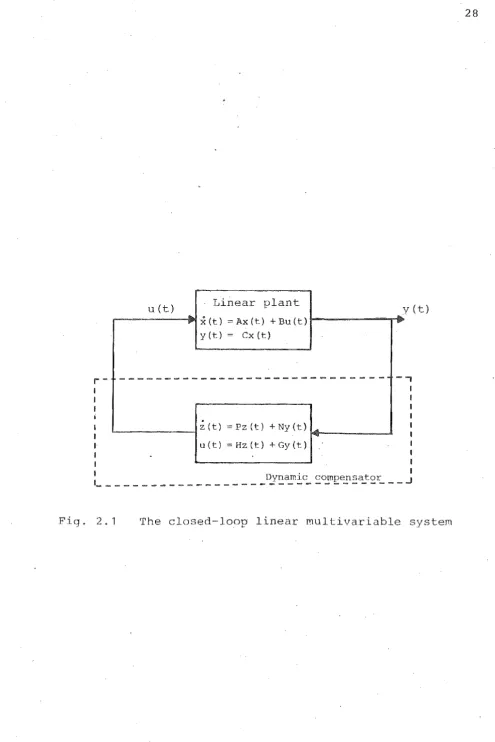
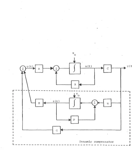
A more direct approach is that adopted by Levine and Athans [3] and generalized by Johnson and Athans [4]. In this approach, the controller is constrained to be a fixed-configuration (low-order) dynamic system. The complete closed-loop system is then as shown in Fig. 2.1.
The design problem is to find the optimal compensator parameters contained in (P, N, G, H) to minimize the chosen quadratic performance index. The compensator structure shown in Fig. 2.1 is quite general and includes the classical lag- and lead-type compensators, proportional-plus-integral controllers, etc. ~otice that this problem is of the same type as the analytical design problem treated by Newton, Gould and Kaiser [5] and others. However, the classical solution technique via Laplace transforms are oriented towards hand calculations and are only suitable for low order 8180 systems having just a few adjustable parameters. The design of high-order, multi-parameter systems is only feasible via computer-oriented stite-space methods such as those developed in [3], [4].
The algorithm given in [3], [4] for computing the optimal compensator parameters is of the so-called indirect type: the necessary conditions for optimality are derived as a set of equations which are then solved iteratively. Unfortunately, a non-linear algebraic matrix equation .has to be solved at every iteration, and this is computationally expensive. A variant of this algorithm [6] avoids the
solution of non-linear equations but at the risk of divergence.
I
I I I
1
I
u(t)
..
Linear plantx(t) =Ax(t) +Bu(t)
...
y(t) ex (t)
---
---~(t) =Pz(t) + Ny (t) AI
~
u(t) =Hz(t) +Gy(t)
.
y(t)
-"'~
~
-
-, 1I
I I I I
1 I
I
1- _ _ _ _ _ _ _ _ _ _ _ _ _ Dynamic compensator J I
[image:40.568.49.544.30.772.2]
direct type is presented which requires the solution of only linear equations while appearing to exhibit rapid convergence. The approach adopted is to directly minimize the performance index with respect to the compensator
parameters using a gradient technique. Consideration is also given to the elimination of redundant compensator parameters by employing suitable canonical forms so as to minimize wasteful computation. The greatly improved
computational efficiency of the new algorithm should enhance the practical usefulness of this design approach.
All the abovementioned algorithms require an initial guess of compensator parameters that stabilizes the
closed-loop system. If the plant is open-loop stable, clearly there is no problem in doing ·so. However, the choice of such stabilizing compensator parameters becomes difficult if the plant is open-loop unstable. A modi ed form of the direct-type algorithm mentioned earl
circumvents this di f cuI ty is de'scribed in § 2.3.
that
Although only the time-invariant, infinite time regulator problem is considered in this chapter, the results can be extended to the time-varying finite-time case as will be shown in Chapter 3.
2.2 OPTIMAL OUTPUT FEEDBACK PROBLEM,
2.2.1 Problem formulation
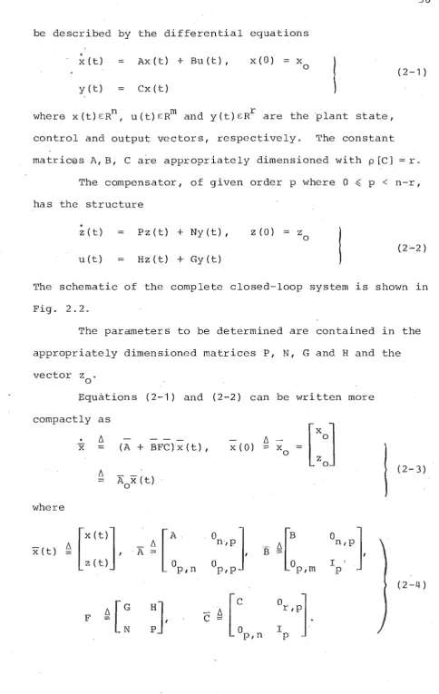
be described by the dif rential equations
·
x(t)
=
Ax(t) + Bu(t), y (t) = Cx (t)x(O) x o
where X(t)ERn, u(t)ERm and y(t)ERr are the ·plant state, control and output vectors, re ctively. The constant
(2-1)
matrices A,B, C are appropriate dimensioned with p [C]
=
r. The compensator, of given order p where 0 ~ p < n-r, has the structure·
z(t)
=
Pz(t)+
Ny(t), u(t) = Hz(t)+
Gy(t)z(O) = z o
The schematic of the complete closed-loop system is shown in Fig. 2.2.
The parameters to be determined are contained in the appropriately dimensioned matrices P, N, G and H and the
vector z . o
EquAtions (2~1) and (2-2) can be written more compactly as
·
tJ.x =
(A+
BFC) x (t) ItJ.
=
AoX (t) where[x(t1
[A
x
(t) tJ. 'A6 0p,n
=
z (t)
:J
tJ.
X (0)
=
°n,p
J
°P/P
[ ::J
x 0
=
~[:p,m
Or,
pJ .
I '
P
°n,p
1
I I P
(2- 3)
[image:42.566.47.532.49.815.2]r
-I I I I I I I I
I I I I
I I
I
L
Fig. 2.2
z (t)
x
o
s
f
x(t)
v
(t)1----.,... ...
- - - I I I
I
I . I . I I
I
Dynamic compensator I
---..1
[image:43.571.67.512.35.542.2]The next step is to find a suitable performance index the composite system (2-3), Suprose the following quadratic performance index is used,
J (F)
!
J
00 X I (t)Qx (
t) + u '( t) R 1 u ( t ) +~
i (t) R2~
(t) d to .
where Q ~ 0, R1 > 0 and R2 > O. Then from (2-3) and (2 4),
and where
=.1
fro
X i (t) [Q+
C iF'.a
o
]x(t)dt (2-6 )
(2-7 )
Notice that in (2-5), quadratic weightings are placed not onlY'on x(t) but so on the plant and 'compensator inputs; u(t), ~(t). This is in order to limit the compensator gains so as to satisfy physical constraints and also to limit
noise transmis on. The integrand in (2-5) differs slightly, though not materially, from that adopted in [4].
Now om {2-3},
x(t} = ¢(t,O)x(O)
where ¢(t,O) is the transition matrix given fry
¢ (t,O) :::: e
A t o
Substitution of (2-8) into (2-6) gives
J
(F)(2-8 )
(2-9 )
(2-10)
Problem statement 81
Given the ant (2-1) and the compensator (2-2) of given order p, find the parameter matr F such that
the quadratic formance index (2-10) is minimized. Remarks
(Rn. I t assumed that the compensated system
(2~3) is stable. Otherwise J(F) in (2 10) will become infinite, thus rendering the optimization problem
'meaningless.
(R2). 8 x is, in general, not known exactly, o
i t is impracti to "tune up" z o to match x o· Hence Zo is at rest [4], i.e. Zo
=
o.
(R3) . compensator matrices P, N, G and H must be made independent of x i otherwise every variation
o
on xo' a corresponding change in compensator matrices is required. This can be achieved if i t is supposed that
[4] Xo is
a
random variable with known covariance, i.e., E{x }o
I t:,.
0, E{x x } == X .
0 0 0 (The zero-mean assumption
is made convenience of ana is only.) Then to remove the dependence of the compensator matrices on x
o' new performance index
J(F) E{J(F)}
fine a
(2-11)
Clearly, J(F) so defined is an average measure of
J
for a given distribution of x .o
On titution of (2-10) into the last ssion, noting the independence of Zo on Xo and remarks made in (R2) I
(2-12)
where
X A E{x Xi}
[ ::.n :n.
p
1
(2-13)=
-0 o 0
p,p
whence a new problem statement in place of (8"1) may now be stated.
Problem statement 82
Given the plant (2-1) and the compensator (2-2) of gi ven order P, 0.(, P < n-r, find the parameter matrix F
such that the performance index (2-12) is minimized.
This is obviouslY a parameter optimization problem. The necessary conditions that must be sa sfied by the optimal solution will be derived later in §2.2.3.
2.2.2 Canonical s for P and N
The parameter matrix F defined in the compensator
(2 -2) has a total of (p + m) x (p + r) elements. However, in
view of the fact that the compensator state z is arbitrary to within a (non-singular) linear transformati~n, p2 of these elements are redundant. Thus, an upper bound on the number of independent parameters is given by
(p+m)x(p+r) p2
=
pm + pr + mr (2-14)Iri [4] and [10], the fa~t that there are redundancies in F has not been mentioned. It would advantageous, although not essential, to adopt
a
canonical form for the compensatorThis is in order to limit the dimensionality of the parameter optimization problem. Unfortunately, there is no such canonical form for MIMO systems that does not require some prior knowledge of the system.
For instance, if the structural indices of the optimal compensator (2 2) are known beforehand (of course they are not!), then the Bucy-Ackermann canonical form [8] may be used. The same problem arises in the identi cation of systems in state-variable form [30].
Notwithstanding these difficulties, i t will now be shown that if the following (very mild) assumption is made, the elimination of p2 - P redundant parameters becomes possible.
Assumption
(Al). The optimal compensator matrix P is cyclic (this is even milder than assuming that the optimal P has distinct eigenvalues):
There no further loss of generality in assuming P is in the companion form:
0 1 0 'u • <» 0
0 0 1 0
P
=
(en
0 0 0 1
x x x x
If so desired, the remaining p r~dundant parameters may be eliminated by making the following stronger
Assumption
(A2). The optimal compensator (2-2) is completely controllable by at least one its inputs y .. Subsequently,
1
by suitable numbering of the elemen~s in y, i t will be assumed that one such input is the first element of y. Notice that assumption (A2) implies, but is not implied by, assumption (A1).
Then, with Pin the 'form (C1), there is no further loss of genera ty in letting the first column N be the constant vector (0, 0, . . . , 0, 1) I i . e. ,
0 x x 0 x x
N =:; (C2 )
0 x x 1 x x
It may be verified that the canonical forms (C1) and (C2) result. ln a compensator that has the reduced number of parameters (2 14). However, as stated'earlier, 'it is not essential that either of the foregoing assumptions (A1) and
(A2) be made. These assumptions have the bene cial effect of reducing the dimensionality of the parameter optimization problem but at the risk of obtaining a less than optimal solution.
2.2.3 Main results
Then,.
Theorem 1
Given the 1 ar differential system
~ (t)
=
M x (t),t1
i
Jt Xl (t) Rx(t)dto
J,. Xl K(t )x 2 0 0 0
(T1-1)
(T1 2)
where K(o) is the symmetric, positive-definite matrix
t .
K(t) :::::
f
t1
<I>' (T,t) R<I>(T,t)dT
<I>(t,t } is the tran tion matrix of
o (T1-1). Also,
K(t} satisfies the matrix differential equation
-K(t)
=
MIK(t)+
K(t)M+
Rwith boundary condition
Corollary
If M is stable, then
i
[00
Xi (t)R x(t)dto
.
=
i
Xl o Kx 0and K satisfies the Lypunov equation
o
=
M'K+
KM+
R(T 1-3)
(T1 4)
(T1 -5)
(T1 6)
Identify A in (2~3) with M in (T1-1) and Q
+
IF' o. in (2 12) with R in (T1 5), then
where K satisfies the Lypunov equation
o
=
'F'RFC (2-16)Hence, the problem becomes one of minimizing J in (2-15) with respect,to F subject to the constraint (2 16). From
(2 15) and (2 -16) , the Lagrang L, thus
L
!
tr {KX } + ;!,. tr {(A' K
+ KA + Q + C IF' RFC) L' }, 0 2 0 0 (2-17)
where L is the (n + p) x (n
+
p) Lagrange multipl matrix defined by'dL
'dK
=
A o L + LA' + 0o
(2-18)Then, the expression for the gradient of J with respect to F is
'dJ
'dF
=
, + B' (2-19)Remarks
(R4). Similar expressions have also been derived in
[4] I [10] for constant dynamic compensators u ng an
extension of [3]. In [3], an application Kleinman's
A
t lemma [11] to J so that a f st order expan on of e 0 isobtained. The de vation is, however, much more involved than that shown above, which is similar to that proposed recently in [12].
(R5). Consider the design of constant gain
controller (i.e., p
=
0) and C is non-singular, e.g., C Then is readily seen that results obtained above become the neces and s f ient condition for· the optimal linear state feedback solution ved by Kalman[ 1
I .
Equations (2 15), (2~16), (2-18) and (2-19) provide suff ient information for the minimization of J to be performed. To this end, several algorithms have been proposed, see e.g. [6]. These are discussed in the next section
2.2.4 Solution thIns
All the sting solution algorithms for the problem (52) are iterative in nature. Each search is initialized with a guessed value F such that (2-3) is closed-loop stable. After this, the procedure that is employed to
obtain the optimal solution belongs to one of the following two types.
2.2.4.1 Indirect
When (2 19) is set to zero, then
F =
which is a necessary' condition for optimality. Any computational method which uses equation (2-20) in
(2-20)
conjunction with (2-15), (2-16) and (2-18) known as an
indirect-type algorithm.
The first indirect-type.computational algor hm is that suggested in [3]. After a stabilizing F has been chosen to initialize the. search, K is then obtained from
(2-16). Substitution of F (still unknown) trom (2 20) into
(2-18) with known K results in'a non-linear equation with L
iteration. It has been shown [3] that in this way J will crease monotonically. However, to obtain the solution of the non-linear equation for Lat every iteration is exceedingly time-consuming.
The method suggested in [6] is a variant of the above algorithm in that for a given F, K and L are
solved using (2-16) and (2-18) respectively. These are then substituted into (2-20) to obtain a new F to complete an ration. In this way, the solution of non-linear equation is avoided. Unfortunately, experience has shown
that this indirect algorithm is' computationally unsatisfactory for there always exists the risk of divergence.
2.2.4.2 Direct type
A new computational procedur~ of the direct-type will now be described. It was first proposed by Choi and Siiisena [7]. A similar approach can also be found in a later pUblication by Horisberger and Belanger [14].
The essential difference between the proposed method in [7] and the indirect-type methods discussed earlier is that instead of setting (2-19) to zero as has been done in §2.2.4;', the explic expressions for J and dJ/aF are now used in a gradient-type function minimization technique such as that of Davidon-Fletcher-Powell (DFP) [15], see Appendix A. I The optimal F is
therefore determined by direct minimization of J.
Step (i):
Step (ii):
compute K, L using (2 16) and (2 18) respe ly.
The cost
J,
gradientaJ/aF
are obtained using(2~15) and (2-19) respectively.
Step ( i): Update F in accordance with the rules of the gradient algorithm used. Terminate search if
"oF11
orII
aJ/aFII
is smaller than some prescribed tolerance. Otherwise return to (i).Remarks
(R6). No that for fixed F, the computation of J
and
aJ/aF
only requires the solution of linear equations (2-16) and (2-18). Several methods are available to solve equations of this type, see e.g. [16]-[18].(R7). All ues of F tried during the subsequent
unidirectional searches in step (iii) above must also stabilize the closed-loop system (2~3). Now, because of the positiveness the in~egrand in (2-J2), i t is evident that J + 00 as F approaches the stability boundary. Hence,
in view of the fact that the derivative of J exists, a minimum of J must occur before the stability boundary is encountered. There remains the possibility that too large a taken during the initial stages of the search could take F into the unstable region. However, this can be
avoided by subjecting the value of F to a Hurwitz stability test (see e.g. [19]) although computational evidence
indicates that such
a
precaution is not usually necessary.(R8). If canonical forms (C1) and (C2) in §2.2 2
gradient matr (aJ/dF) for use in the iterative search. The components of aJ/aF corresponding to the fixed
compensator parameters (the ones or zeros) may be
disregarded. In this way, the total number of parameters which need to be considered in the min zation procedure is equal to pm + mr + pro The computational efficiency is there enhanced.
(R9). It is conceivable that several local optimal solutions may exist because J is, in general, a non-convex function F. Hence, irrespective what algorithm is employed, iterations should be commenced for different priming values of F.
2.2.5 Numerical example
The numerical example is taken from [20] and refers to a Mach 2.7 flight condition of a supersonic transport aircraft. The system equations are
.
x -.037 O. -6.37 1.25 .0123 O. O. O. .00055 1.0 -.23 .016 -1.0 O. .0618 .0457x +
.00084 O . .08 -.0862 .000236 O. .804 :....0665 u
Suppose a constant gain feedback controller (p
=
0) to be constructed using only the last three state variab s,i.e. C [03,1 13 ], For Q
=
14 , R=
12 and Xo=
14 , thefeedback gains converged after 35 iterations of the DFP algorithm to
3.54
~7'61]
5.06
with the corresponding cost J 79.56. This compares with the priming values F' == O
2
,
3 and J=
15568. The convergence criterion was·2.3 OPTIMAL OUTPUT FEEDBACK CONTROLS FOR UNSTABLE PLANTS
In this section, the design of constant-gain output dback controllers for unstable plants is considered. The extension of the results to the design of dynamic compensators of the. form (2-3) is straightforward. The results obtained in this section first appeared in a paper by Choi and Sirisena [31].
Problem statement S3 Given the plant
Ax (t) + Bu (t) , x(O) == Xo
(2-21) yet) == C~(t)
where X(t)£Rn, u(t)£Rm and y(t)£Rr , find the constant matrix such that
u(t) Fy(t) minimizes the performance index
J =
{ Joo
X I (t) Qx (t)+
u I (t) Ru (t) d t},o
(2-22)
Q~O, R>O (2-23)
It is assumed as in (R3) that x
o is a random variable with
known covariance, E{x.}
=
0 E{x Xl} == Xo.o ' . 0 0
As has been pointed out earlier, all the iterative techniques described in §2.2.4 require an initiaL guess of F that st.abilizes the clGsed-loop system. If (2 21) is open
loop- stable, then the cho F == 0 suffices.
![Table I [24] where only "approximate" non-interaction is aimed](https://thumb-us.123doks.com/thumbv2/123dok_us/9955326.496875/19.566.50.518.49.822/table-i-approximate-non-interaction-aimed.webp)