Deep Active Learning for Named Entity Recognition

Deep Active Learning for Named Entity Recognition

UT Austin Austin, TX 78712 [email protected]

Hyokun Yun Amazon Web Services

Seattle, WA 98101 [email protected]

Zachary C. Lipton Amazon Web Services

Seattle, WA 98101 [email protected] Yakov Kronrod

Amazon Web Services Seattle, WA 98101 [email protected]

Animashree Anandkumar Amazon Web Services

Seattle, WA 98101 [email protected]

Abstract

Deep neural networks have advanced the state of the art in named entity recogni-tion. However, under typical training pro-cedures, advantages over classical meth-ods emerge only with large datasets. As a result, deep learning is employed only when large public datasets or a large bud-get for manually labeling data is available. In this work, we show that by combining deep learning with active learning, we can outperform classical methods even with a significantly smaller amount of training data.

1 Introduction

Over the past several years, a series of papers have used deep neural networks (DNNs) to advance the state of the art in named entity recognition (NER) (Collobert et al.,2011;Huang et al.,2015; Lam-ple et al., 2016; Chiu and Nichols, 2015; Yang et al.,2016). Historically, the advantages of deep learning have been less pronounced when work-ing with small datasets. For instance, on the pop-ular CoNLL-2003 English dataset, the best DNN model outperforms the best shallow model by only 0.4%, as measured by F1 score, and this is a small dataset containing only 203,621 words. On the other hand, on the OntoNotes-5.0 English dataset, which contains 1,088,503 words, a DNN model outperforms the best shallow model by 2.24% (Chiu and Nichols,2015).

In this work, we investigate whether we can train DNNs using fewer samples under the ac-tive learning framework. Acac-tive learning is the paradigm where we actively select samples to be used during training. Intuitively, if we are able to select the most informative samples for training,

we can vastly reduce the number of samples re-quired. In practice, we can employ Mechanical Turk or other crowdsourcing platforms to label the samples actively selected by the algorithm. Re-ducing sample requirements for training can lower the labeling costs on these platforms.

We present positive preliminary results demon-strating the effectiveness of deep active learn-ing. We perform incremental training of DNNs while actively selecting samples. On the stan-dard OntoNotes-5.0 English dataset, our approach matches 99% of the F1 score achieved by the best deep models trained in a standard, supervised fashion despite using only a quarter

2 NER Model Description

We use CNN-CNN-LSTM model from Yun

(2017) as a representative DNN model for NER. The model uses two convolutional neural networks (CNNs) (LeCun et al., 1995) to encode charac-ters and words respectively, and a long short-term memory (LSTM) recurrent neural network (Hochreiter and Schmidhuber,1997) as a decoder. This model achieves the best F1 scores on the OntoNotes-5.0 English and Chinese dataset, and its use of CNNs in encoders enables faster training as compared to previous work relying on LSTM encoders (Lample et al.,2016;Chiu and Nichols, 2015). We briefly describe the model:

Data Representation We represent each input

sentence as follows. First, special [BOS] and

[EOS]tokens are added at the beginning and the end of the sentence, respectively. In order to batch the computation of multiple sentences, sentences with similar length are grouped together into buck-ets, and[PAD]tokens are added at the end of sen-tences to make their lengths uniform inside of the

Formatted Sentence [BOS] Kate lives on Mars [EOS] [PAD]

Tag O S-PER O O S-LOC O O

Table 1: Example formatted sentence. To avoid clutter,[BOW]and[EOW]symbols are not shown.

bucket. We follow an analogous procedure to rep-resent the characters in each word. For example, the sentence ‘Kate lives on Mars’ is formatted as shown in Table1. The formatted sentence is de-noted as{xij}, wherexij is the one-hot encoding of thej-th character in thei-th word.

Character-Level Encoder For each wordi, we use CNNs to extract character-level featureswchar

i (Figure 1). We apply ReLU nonlinearities (Nair and Hinton, 2010) and dropout (Srivastava et al., 2014) between CNN layers, and include a residual connection between input and output of each layer (He et al.,2016). So that our representation of the word is of fixed length, we apply max-pooling on the outputs of the topmost layer of the character-level encoder (Kim,2014).

wchar 2

h(2)

21 h(2)22 h(2)23 h24(2) h(2)25 h(2)26 h(2)27

h(1)

21 h(1)22 h(1)23 h24(1) h(1)25 h(1)26 h(1)27

x21 x22 x23 x24 x25 x26 x27

[BOW] K a t e [EOW] [PAD] max pooling

Figure 1: Example CNN architecture for Character-level En-coder with two layers.

Word-Level Encoder To complete our rep-resentation of each word, we concatenate its character-level features with wemb

i , a latent word embedding corresponding to that word:

wfull

i := wchari ,wembi

.

In order to generalize to words unseen in the train-ing data, we replace each word with a special

[UNK] (unknown) token with 50% probability

during training, an approach that resembles the word-drop method due toLample et al.(2016).

Given the sequence of word-level input features

wfull

1 ,wfull2 , . . . ,wfulln , we extract word-level repre-sentationshEnc

1 ,hEnc2 , . . . ,hEncn for each word po-sition in the sentence using a CNN. In Figure 2,

we depict an instance of our architecture with two convolutional layers and kernels of width 3. We concatenate the representation at thel-th convolu-tional layerh(_il), with the input featureswfull

i :

hEnc

i =

h(_il),wfull

i

hEnc

1 hEnc2 hEnc3 h4Enc hEnc5 hEnc6 hEnc7

h(2)

1 h(2)2 h(2)3 h4(2) h(2)5 h(2)6 h(2)7

h(1)

1 h(1)2 h(1)3 h4(1) h(1)5 h(1)6 h(1)7

wfull

1 wfull2 w3full w4full wfull5 wfull6 w7full [BOS] Kate lives on Mars [EOS] [PAD]

Figure 2: Example CNN architecture for Word-level Encoder with two layers.

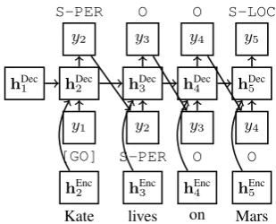
Tag Decoder The tag decoder induces a prob-ability distribution over sequences of tags, con-ditioned on the word-level encoder features:

Py2, y3, . . . , yn−1 |hEnci 1. We use an LSTM RNN for the tag decoder, as depicted in Figure3. At the first time step, the [GO]-symbol is

pro-vided as y1 to the decoder LSTM. At each time

stepi, the LSTM decoder computeshDec

i+1, the

hid-den state for decoding wordi+ 1, using the last tagyi, the current decoder hidden statehDeci , and the learned representation of next wordhEnc

i+1.

Us-ing a softmax loss function,yi+1 is decoded; this

is further fed as an input to the next time step. While it is computationally intractable to find the best sequence of tags with an LSTM decoder, Yun (2017) reports that greedily decoding tags from left to right often yields performance supe-rior to chain CRF decoder (Lafferty et al.,2001), for which exact inference is tractable.

1_y

S-PER O O S-LOC

y2 y3 y4 y5

hDec

1 hDec2 hDec3 hDec4 hDec5

y1 y2 y3 y4

[GO] S-PER O O hEnc

2 hEnc3 hEnc4 hEnc5 Kate lives on Mars

Figure 3: LSTM architecture for Tag Decoder.

3 Active Learning

As with most tasks, labeling data for NER usually requires manual annotations by human experts, which are costly to acquire at scale. Active learn-ing seeks to ameliorate this problem by strategi-cally choosing which examples to annotate, in the hope of getting greater performance with fewer annotations. To this end, we consider the follow-ing setup for interactively acquirfollow-ing annotations. The learning process consists of multiple rounds: At the beginning of each round, the active learn-ing algorithm chooses sentences to be annotated up to the predefined budget. After receiving anno-tations, we update the model parameters by train-ing on the augmented dataset, and proceeds to the next round. We assume that the cost of annotating a sentence is proportional to the number of words in the sentence, and that every word in the selected sentence needs to be annotated; the algorithm can-not ask workers to partially ancan-notate the sentence. While various existing active learning strategies suit this setup (Settles,2010), we explore the un-certainty sampling strategy, which ranks unlabeled examples in terms of current model’s uncertainty on them, due to its simplicity and popularity. We consider three ranking methods, each of which can be easily implemented in the CNN-CNN-LSTM model as well as most common models for NER.

Least Confidence (LC):This method sorts ex-amples in descending order by the probability of

not predicting the most confident sequence from the current model (Lewis and Gale,1994;Culotta and McCallum,2005):

1− max

y1,...,ynP[y1, . . . , yn| {xij}]. (1)

Since exactly computing (1) is not feasible with the LSTM decoder, we approximate it with the

probability of a greedily decoded sequence.

Maximum Normalized Log-Probability (MNLP):Our preliminary analysis revealed that the LC method disproportionately selects longer sentences. Note that sorting unlabeled examples in descending order by (1) is equivalent to sorting in ascending order by the following scores:

max

y1,...,ynP[y1, . . . , yn| {xij}]

⇔ max

y1,...,yn

n Y

i=1

P[yi |y1, . . . , yn−1,{xij}]

⇔ max

y1,...,yn

n X

i=1

logP[yi|y1, . . . , yn−1,{xij}]. (2)

Since (2) contains summation over words, LC

method naturally favors longer sentences. Be-cause longer sentences require more labor for an-notation, however, we find this undesirable, and propose to normalize (2) as follows, which we call Maximum Normalized Log-Probability method:

max

y1,...,yn

1

n

n X

i=1

logP[yi |y1, . . . , yn−1,{xij}].

Bayesian Active Learning by Disagreement (BALD): We also consider the Bayesian

met-ric proposed by Gal et al. (2017). Denote

P1_,P2_{, . . .P}M _{as models sampled from the} pos-terior. Then, one measure of our uncertainty on the ith word is fi, the fraction of models which disagreed with the most popular choice:

fi = 1−maxy

_{m: argmaxy0P}m_[y

i=y0] =y

M ,

where|·|denotes cardinality of a set. We normal-ize this by the number of words as 1

n P_n

j=1fj, and sort sentences in decreasing order by this score. FollowingGal et al.(2017), we used Monte Carlo dropout (Gal and Ghahramani, 2016) to sample from the posterior, and setMas 100.

4 Experiments

0 20 40 60 80 70

75 80 85

Percent of words annotated

Test

F1

score MNLP

LC BALD RAND Best Deep Model Best Shallow Model

(a) OntoNotes-5.0 English

0 20 40 60 80 100 65

70 75

Percent of words annotated

Test

F1

score MNLP

LC BALD RAND Best Deep Model Best Shallow Model

(b) OntoNotes-5.0 Chinese Figure 4: F1 score on the test dataset, in terms of the number of words labeled.

nw bc tc wb bn mz

0 100 200 300 400 500

#

half_data, F1=85.10 no_nw_data, F1=81.49 nw_only_data, F1=82.08

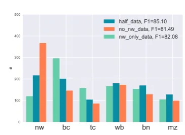
Figure 5: Genre distribution of top 1,000 sentences chosen by an active learning algorithm

Comparisons of selection algorithms We em-pirically compare selection algorithms proposed in Section 3, as well as uniformly random base-line (RAND). All algorithms start with an iden-tical 1% of original training data and a randomly initialized model. In each round, every algorithm chooses sentences from the rest of the training data until 20,000 words have been selected, adding this data to its training set. Then, the algorithm up-dates its model parameters by stochastic gradient descent on its augmented training dataset for 50 passes. We evaluate the performance of each al-gorithm by its F1 score on the test dataset.

Figure 4shows results. All active learning al-gorithms perform significantly better than the

ran-dom baseline. Among active learners, MNLP

slightly outperformed others in early rounds. Im-pressively, active learning algorithms achieve 99% performance of the best deep model trained on full data using only 24.9% of the training data on the English dataset and 30.1% on Chinese. Also, 12.0% and 16.9% of training data were enough for deep active learning algorithms to surpass the

performance of the shallow models fromPradhan

et al.(2013) trained on the full training data.

Detection of under-explored genres To better understand how active learning algorithms choose informative examples, we designed the following experiment. The OntoNotes datasets consist of six genres: broadcast conversation (bc), braod-cast news (bn), magazine genre (mz), newswire (nw), telephone conversation (tc), weblogs (wb). We created three training datasets: half-data, which contains random 50% of the original train-ing data,nw-data, which contains sentences only from newswire (51.5% of words in the original data), andno-nw-data, which is the complement ofnw-data. Then, we trained CNN-CNN-LSTM model on each dataset. The model trained on

half-dataachieved 85.10 F1, significantly outper-forming others trained on biased datasets ( no-nw-data: 81.49,nw-only-data: 82.08). This showed the importance of good genre coverage in training data. Then, we analyzed the genre distribution of

1,000 sentencesMNLPchose for each model (see

Figure5). For no-nw-data, the algorithm chose many more newswire (nw) sentences than it did for unbiasedhalf-data(367 vs. 217). On the other hand, it undersampled newswire sentences for nw-only-dataand increased the proportion of broad-cast news and telephone conversation, which are genres distant from newswire. Impressively, al-though we did not provide the genre of sentences to the algorithm, it was able to automatically de-tect underexplored genres.

5 Conclusion

References

Jason PC Chiu and Eric Nichols. 2015. Named

en-tity recognition with bidirectional lstm-cnns. arXiv

preprint arXiv:1511.08308.

Ronan Collobert, Jason Weston, L´eon Bottou, Michael Karlen, Koray Kavukcuoglu, and Pavel Kuksa. 2011. Natural language processing (almost) from

scratch. Journal of Machine Learning Research

12(Aug):2493–2537.

Aron Culotta and Andrew McCallum. 2005. Reduc-ing labelReduc-ing effort for structured prediction tasks. In

AAAI. volume 5, pages 746–51.

Yarin Gal and Zoubin Ghahramani. 2016. A theoret-ically grounded application of dropout in recurrent

neural networks. InAdvances in Neural Information

Processing Systems. pages 1019–1027.

Yarin Gal, Riashat Islam, and Zoubin Ghahramani. 2017. Deep bayesian active learning with image

data.arXiv preprint arXiv:1703.02910.

Kaiming He, Xiangyu Zhang, Shaoqing Ren, and Jian Sun. 2016. Deep residual learning for image

recog-nition. In Proceedings of the IEEE Conference

on Computer Vision and Pattern Recognition. pages 770–778.

Sepp Hochreiter and J¨urgen Schmidhuber. 1997.

Long short-term memory. Neural computation

9(8):1735–1780.

Zhiheng Huang, Wei Xu, and Kai Yu. 2015.

Bidirec-tional lstm-crf models for sequence tagging. arXiv

preprint arXiv:1508.01991.

Yoon Kim. 2014. Convolutional neural

net-works for sentence classification. arXiv preprint

arXiv:1408.5882.

John Lafferty, Andrew McCallum, Fernando Pereira, et al. 2001. Conditional random fields: Probabilis-tic models for segmenting and labeling sequence

data. InProceedings of the eighteenth international

conference on machine learning, ICML. volume 1, pages 282–289.

Guillaume Lample, Miguel Ballesteros, Sandeep Sub-ramanian, Kazuya Kawakami, and Chris Dyer. 2016. Neural architectures for named entity recognition.

arXiv preprint arXiv:1603.01360.

Yann LeCun, Yoshua Bengio, et al. 1995. Convolu-tional networks for images, speech, and time series.

The handbook of brain theory and neural networks

3361(10):1995.

David D Lewis and William A Gale. 1994. A

sequen-tial algorithm for training text classifiers. In

Pro-ceedings of the 17th annual international ACM SI-GIR conference on Research and development in in-formation retrieval. Springer-Verlag New York, Inc., pages 3–12.

Vinod Nair and Geoffrey E Hinton. 2010. Rectified linear units improve restricted boltzmann machines. InProceedings of the 27th international conference on machine learning (ICML-10). pages 807–814. Sameer Pradhan, Alessandro Moschitti, Nianwen Xue,

Hwee Tou Ng, Anders Bj¨orkelund, Olga Uryupina, Yuchen Zhang, and Zhi Zhong. 2013. Towards

ro-bust linguistic analysis using ontonotes. InCoNLL.

pages 143–152.

Burr Settles. 2010. Active learning literature survey.

University of Wisconsin, Madison52(55-66):11. Nitish Srivastava, Geoffrey E Hinton, Alex Krizhevsky,

Ilya Sutskever, and Ruslan Salakhutdinov. 2014. Dropout: a simple way to prevent neural networks

from overfitting. Journal of Machine Learning

Re-search15(1):1929–1958.

Zhilin Yang, Ruslan Salakhutdinov, and William Co-hen. 2016. Multi-task cross-lingual sequence

tag-ging from scratch. arXiv preprint arXiv:1603.06270

.