1. Determine the impulse responses for the following systems: a) 2( t

ECE 300

Signals and Systems Homework 4

Due Date: Tuesday September 29 at the beginning of class

Exam 1, Thursday October 1 Problems

1. Determine the impulse responses for the following systems:

a) 2( )

( ) ( ) ( )

t t

y t x t e− −λ x λ λd −∞

= +

∫

1 ( )

( ) ( 2)

t t

y t e λ x λ dλ −

− − −∞

=

∫

c) 2 (y t )−y t( )=3 (x t+2) d) ( ) 1 ( ) t

t M

y t x d

M ₋ λ λ

=

_∫

2. Consider the following two subsystems, connected together to form a single LTI system.

1( )

h t v t( ) y t( )

( )

x t

2( ) h t

Determine the impulse response of the entire system if the impulse responses of the subsystems are given as:

( )

h t

a) ₁( ) ( ) ₂( ) 2 t ( )

h t =δ t h t = e u t−

b) h t₁( )=e u t−t ( ) h t₂( )=2 (δ t−1)

−

t u t

c) ( 1) ( 1)

1( ) ( 1) 2( ) ( 1)

t t

t e u t h t e u

h = − + + = − − t

d) h1( )t =u t( )−u t( −1) h2( )= ( )

3. Consider a causal linear time invariant system with impulse response given by ( 1)

( ) t ( 1)

h t =e− − u t− The input to the system is given by

( ) ( ) ( 1) ( 3)

x t =u t −u t− +u t−

Using graphical convolution, determine the outputy t( ) for 2≤ ≤t 5. Note the limited range of t we are interested in !

Specifically, you must

a) Flip and slideh t( )

b) Show graphs displaying both h t( −λ) and x( )λ for each region of interest c) Determine the range of t for which each part of your solution is valid d) Set up any necessary integrals to compute y t( )

e) Evaluate the integrals

You should get (in unsimplified form)

( 1) 1

( 1) 1 ( 1) 1 3

[ 1] 2

( )

[ 1] [ ] 4

t

t t t

e e t

y t

e e e e e t

− −

− − − − −

⎧ 4

5

− ≤ ≤

= ⎨

− + − ≤

⎩ ≤

4. Consider a causal linear time invariant system with impulse response given by ( 1)

( ) t ( 1)

h t =e− − u t−

a) Show that the step response of the system (the response to a unit step) is ( 1)

( ) [1 t ] ( 1)

s t e u t

y = − − − −

b) Using linearity and time-invariance, determine the response of the system to the input

( ) ( 1) 2 ( 2)

x t =u t− − u t−

c) Use graphical convolution to determine the output of the system. d) Show that your answers to b and c are the same.

5. Consider a causal linear time invariant system with impulse response

2

( ) 1 0.5 [ ( 2) ( 1)]

h t = −⎡_⎣ t ⎤_⎦ u t+ −u t−

The input to the system is

( ) ( 1) ( 1) 2 ( 2) 2 ( 3)

x t =u t+ −u t− − u t− + u t−

These two functions are plotted below:

-4 -3 -2 -1 0 1 2

-1.5 -1 -0.5 0 0.5 1 1.5

Time (sec)

h(t

)

-2 -1 0 1 2 3 4

-2 -1 0 1

Time (sec)

x(

t)

Using graphical convolution, set up the integrals to determine the outputy t( ) Specifically, you must

• Flip and slide h t( )

• Show graphs displaying h t( −λ) relative to x( )λ for each region of interest.

• Determine the ranges of for which each part of your solution is valid. t

• Set up any necessary integrals to compute . Your integrals must be complete and simplified as much as possible (no unit step functions)

( )

y t

6. For the interconnected feedback system below, determine a relationship between the inputx t( ) and the output in terms of and . Your final answer will be of the form

( )

y t h t₁( ) h t₂( )

( ) *[ ( ) ( )] ( ) *[ ( )]

y t δ t +A t =x t B t

You need to determineA t( ) and B t( ).

Hints: e t( )=x t( )−v t( ) and v t( )=y t( ) *h t2( )

7. (Matlab/Prelab Problem) Read Appendix A, then Download Fourier_Sine_Series.m from the class website.

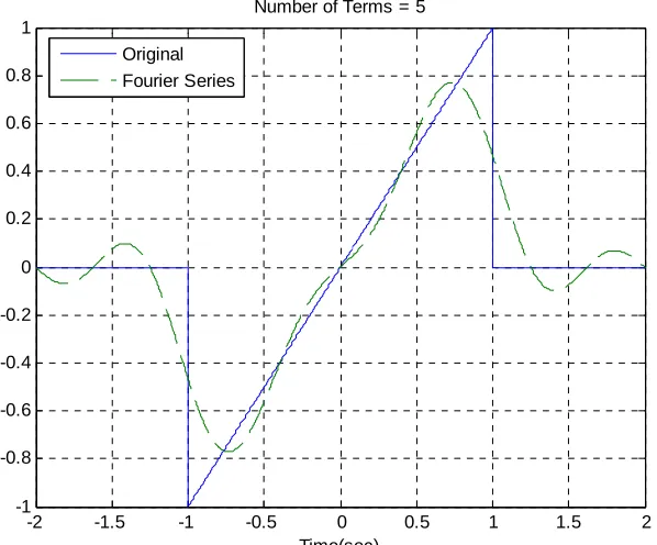
a) If you type (in Matlab’s command line) Fourier_Sine_Series(5) you should get a plot like that shown in Figure 1. As you increase the number of terms in the Fourier series, you should get a better match to the function. Run the code for N=100 and turn in your plot.

b) Copy Fourier_Sine_Series.m to a file named Trig_Fourier_Series.m and implement a full trigonometric Fourier series representation. This means you will have to compute the average value and the , and then use these values in the final estimate.

o

a a_k

c) Using the code you wrote in part c, find the trigonometric Fourier series representation for the following functions (defined over a single period)

Half-wave rectifier (V_m =100 2volts, f₀ =60Hz)

0 0

1

0

0

sin(2 ) 0

2 ( )

0

2 m

V f t t

x

t T T

T t

π ≤ <

=

≤ < ⎧

Full-wave rectifier (V_m =100 2volts, f₀ =60Hz)

0 0

| sin(2 )

( ) _m f t |0 t

x t =V π ≤ ≤T

Use N = 11 and turn in your plots for each of these functions. Also, turn in your Matlab program for one of these.

Figure 1. Trigonometric Fourier series for problem 3.

-2 -1.5 -1 -0.5 0 0.5 1 1.5 2

-1 -0.8 -0.6 -0.4 -0.2 0 0.2 0.4 0.6 0.8 1

Time(sec) Number of Terms = 5 Original

Appendix A

In DE II you learned about representing periodic functions with a Fourier series using trigonometric functions (sines and cosines). In this appendix we will determine how to determine a Fourier sine series series for an odd periodic function using our knowledge of numerical integration in Matlab. The only new thing we will need is the idea of a loop.

Trigonometric Fourier Series If x t( ) ( )

is a periodic function with fundamental period T, then we can represent x t as a Fourier series

0

1 1

( ) _kcos( _o ) _ksin( )

k k

o

x t a a kω t b kω t

∞ ∞

= =

= +

∑

∑

where _o 2

T π

ω = is the fundamental period, is the average (or DC, i.e. zero

frequency) value, and

o a

1 ( )

2

( ) cos( )

2

( ) sin( )

o _T

k _T o

k o

T

a x t dt T

a x t k t

T

b x t k t

T

ω ω

=

=

=

∫

∫

∫

dt

dt

Even and Odd Functions Recall that a function x t( ) is even if x t( )= −x( t) (it is symmetric about the y-axis) and is odd if x(− = −t) x t( )(it is antisymmetric about the y-axis). If we know in advance that functions are even or odd, we can determine that some of the Fourier series coefficients are zero. Specifically,

Ifx t( ) is even all of the bk are zero.

Ifx t( ) is odd all of the a_k (including a_o) are zero.

For Loops Let’s assume we want to generate the coefficients ₂

1 k

k b

k =

+ for k =1

to k=10. One way of doing this in Matlab is by using the following for loop

for k=1:10

In this loop, the variable k first takes the value of 1 until the end is reached, then the value 2, all the way up to k = 10. In this loop we are assigning the coefficients to the array b, hence b(1) = b₁, b(2) = b₂, etc.

Similarly, if we wanted to generate the coefficients 1 1 k

a k =

+ and 2

2 1 k

b k =

+ for

to , we could do this using for loops as follows: 1

k= k=5

for k=1:5

a(k) = 1/(k+1); b(k) = 2/(k^2+1); end;

Note that Matlab requires the indices in an array to start at 1, and that for loops should usually be avoided in Matlab if possible since they are usually less efficient (Matlab is designed for vectorized operations).

Fourier Sine Series Now we want to generate the Fourier series for the periodic function

0 2

( ) 1 1

0 1 2

t

x t t t

t 1

− ≤ < − ⎧

⎪

=_⎨ − ≤ <

⎪ _{≤ <}

⎩

%

% This routine implements a trigonometric Fourier Sine Series %

% Inputs: N is the number of terms to use in the series %

function Fourier_Sine_Series(N)

%

% one period of the function goes from low to high %

low = -2; high = 2;

%

% the difference between low and high is one period %

T = high-low; w0 = 2*pi/T;

%

% the periodic function... %

x = @(t) 0.*(t<-1) + t.*((-1<=t)&(t<1)) + 0.*(t>=1);

%

% find b(1) to b(N) %

for k = 1:N

arg = @(t) x(t).*sin(k*w0*t); b(k) = (2/T)*quadl(arg,low,high);

end;

%

% determine a time vector over one period %

t = linspace(low,high,1000);

%

% find the Fourier series representation %

est = 0;

for k=1:N

est = est + b(k)*sin(k*w0*t);

end;

%

% plot the results %

plot(t,x(t),'-',t,est,'--'); grid; xlabel('Time(sec)');

legend('Original','Fourier Series','Location','NorthWest');