ECE 300 Signals and Systems

ECE 300

Signals and Systems

Homework 5

Due Date: Thursday, April 9, 2009 at the beginning of class

Problems

1. For the following system models, determine if the model represents a BIBO stable system. If the system is not BIBO stable, give an inputx t( ) that

demonstrates this.

a) ( ) ( ( ) 5) t

y t x λ dλ

−∞

=

∫

( ) y t

x t

⎛ ⎞

= _{⎜ ⎟}

⎝ ⎠

c) y t( )=e−x t( ) d) y t( )=x t( )+y t x t( ) ( )

2. For LTI systems with the following impulse responses, determine if the system is BIBO stable.

a) h t( )=e u t−t ( ) b) h t( )=u t( ) c) h t( )=u t( )−u t( −10) d) h t( )=δ(t−1) e) h t( )=sin( ) ( )t u t f) h t( )=e u t−t2 ( ) (hint: use your answer to a)

3. In this problem we will determine the trigonometric Fourier Series for a full wave rectified signal.

a. Using Euler’s identity, show that sin( ) cos( ) 1sin( ) 1sin( )

2 2

α β = α β+ − β α−

and sin( ) sin( ) 1cos( ) 1cos( )

2 2

α β = α β− − α +β

b. Show that for sin 0 0 ₀

2

( ) _m t

x t V ⎛_⎜ω ⎞ ≤ ≤_⎟ t T

⎝ ⎠

4. (Matlab/Prelab Problem) Read Appendix A, then Download Fourier_Sine_Series.m from the class website.

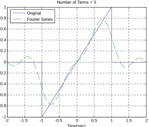
a) If you type (in Matlab’s command line) Fourier_Sine_Series(5) you should get a plot like that shown in Figure 1. As you increase the number of terms in the Fourier series, you should get a better match to the function. Run the code for N=100 and turn in your plot.

b) Copy Fourier_Sine_Series.m to a file named Trig_Fourier_Series.m and implement a full trigonometric Fourier series representation. This means you will have to compute the average value and the , and then use these values in the final estimate.

o

a a_k

c) Using the code you wrote in part c, find the trigonometric Fourier series representation for the following functions (defined over a single period)

Half-wave rectifier (Vm =100 2volts, f0 =60Hz)

0 0

1

0

0

sin(2 ) 0

2 ( )

0

2

m

V f t t

x

t T T T

t

π ≤ <

=

≤ < ⎧

⎪⎪ ⎨ ⎪ ⎪⎩

Full-wave rectifier (V_m =100 2volts, f₀ =60Hz)

0 0

| sin(2 ) ( ) _m f t |0 t

x t =V π ≤ ≤T

(Note that this is not the form of the function we used in problem 3, but this form gives a better idea of what a full-wave rectifier does)

-2 -1.5 -1 -0.5 0 0.5 1 1.5 2 -1

-0.8 -0.6 -0.4 -0.2 0 0.2 0.4 0.6 0.8 1

Time(sec) Number of Terms = 5

Original

Fourier Series

Figure 1. Trigonometric Fourier series for problem 3.

5. (Matlab/Prelab Problem)Read Appendix B and then do the following:

a) Copy the file Trigonometric_Fourier_Series.m to file

Complex_Fourier_Series.m.

b) Modify Complex_Fourier_Series.m so it computes the average value c_o c) Modify Complex_Fourier_Series.m so it directly computes for to

. You are

k

c k =1

e) Using the code you wrote in part d, find the complex Fourier series representation for the following functions (defined over a single period)

1( ) ( ) 0 3 t

f t =e u t− ≤ <t

2

0 2

( ) 3 2 3

0 3 4

t t

f t t

t

≤ < ⎧

⎪

=_⎨ ≤ <

⎪ _{≤ <}

⎩

3

0 2

1 1

( )

3 2 3

0 3 4

t t f t

t t

1 2

− ≤ < − ⎧

⎪ _{− ≤ <}

⎪

= ⎨ _{≤ <}

⎪

⎪ _{≤ <}

⎩

Appendix A

In DE II you learned about representing periodic functions with a Fourier series using trigonometric functions (sines and cosines). In this appendix we will determine how to determine a Fourier sine series series for an odd periodic function using our knowledge of numerical integration in Matlab. The only new thing we will need is the idea of a loop.

Trigonometric Fourier Series If x t( ) ( )

is a periodic function with fundamental period T, then we can represent x t as a Fourier series

0

1 1

( ) _kcos( _o ) _ksin( )

k k

o

x t a a kω t b kω t

∞ ∞

= =

= +

∑

∑

where _o 2

T

π

ω = is the fundamental period, is the average (or DC, i.e. zero

frequency) value, and

o a

1 ( ) 2

( ) cos( ) 2

( ) sin( )

o _T

k _T o

k o

T

a x t dt

T

a x t k t

T

b x t k t

T

ω ω

=

=

=

∫

∫

∫

dt dt

Even and Odd Functions Recall that a function x t( ) is even if x t( )= −x( t) (it is symmetric about the y-axis) and is odd if x(− = −t) x t( )(it is antisymmetric about the y-axis). If we know in advance that functions are even or odd, we can determine that some of the Fourier series coefficients are zero. Specifically,

Ifx t( ) is even all of the bk are zero.

In this loop, the variable k first takes the value of 1 until the end is reached, then the value 2, all the way up to k = 10. In this loop we are assigning the coefficients to the array b, hence b(1) = b₁, b(2) = b₂, etc.

Similarly, if we wanted to generate the coefficients 1

1 k

a k

=

+ and 2

2 1 k

b k

=

+ for

to , we could do this using for loops as follows:

1

k= k=5

for k=1:5

a(k) = 1/(k+1); b(k) = 2/(k^2+1); end;

Note that Matlab requires the indices in an array to start at 1, and that for loops should usually be avoided in Matlab if possible since they are usually less efficient (Matlab is designed for vectorized operations).

Fourier Sine Series Now we want to generate the Fourier series for the periodic function

0 2

( ) 1 1

0 1 2

t

x t t t

t 1

− ≤ < − ⎧

⎪

=_⎨ − ≤ <

⎪ _{≤ <}

⎩

%

% This routine implements a trigonometric Fourier Sine Series %

% Inputs: N is the number of terms to use in the series %

function Fourier_Sine_Series(N)

%

% one period of the function goes from low to high %

low = -2; high = 2;

%

% the difference between low and high is one period %

T = high-low; w0 = 2*pi/T;

%

% the periodic function... %

x = @(t) 0.*(t<-1) + t.*((-1<=t)&(t<1)) + 0.*(t>=1);

%

% find b(1) to b(N) %

for k = 1:N

arg = @(t) x(t).*sin(k*w0*t); b(k) = (2/T)*quadl(arg,low,high); end;

%

% determine a time vector over one period %

t = linspace(low,high,1000);

%

% find the Fourier series representation %

est = 0; for k=1:N

est = est + b(k)*sin(k*w0*t); end;

%

% plot the results %

Appendix B

In the majority of this course we will be using the complex (or exponential) form of the Fourier series, since it is really easier to do various mathematical things with it once you get used to it.

Exponential Fourier Series If x t( ) (

is a periodic function with fundamental period T, then we can represent x t) as a Fourier series

( ) jk ot k k

x t c e ω

∞

=−∞

=

∑

where _o 2

T

π

ω = is the fundamental period, is the average (or DC, i.e. zero

frequency) value, and

o c

o 0 1

c (

T ) x t dt T

=

∫

0 1

( ) o T

jk t k

c x t e

T

ω −

=

∫

Ifx t( )is a real function, then we have the relationships |c_k | |= c_−k | (the magnitude

is even) and (the phase is odd). Using these relationships we can

then write

k c₋ = −

( (c_k

k 1

( ) _o 2 | _k | cos( _o ) k

x t c c kω t c

∞

=

= +

∑