Distributed AdaBoost Extensions for Cost-sensitive
Classification Problems
Ankit Desai
School of Engineering and Applied Science Ahmedabad University
Ahmedabad, India
Sanjay Chaudhary
School of Engineering and Applied Science Ahmedabad University
Ahmedabad, India
ABSTRACT
In data mining, classification of data has always been an area of in-terest and this is especially true after the rapid increase in availabil-ity of data being collected. Cost-sensitive classification is a subset of the broader classification problem where the focus is on solving the class imbalance problem. This paper addresses the class imbal-ance problem using Cost-sensitive Distributed Boosting (CsDb). CsDb is a meta-classifier designed to solve the class imbalance problem for big data, is based on the concept of MapReduce. The focus of this work is to solve the class imbalance problem for the size of data which is beyond the capacity of standalone commod-ity hardware to handle. CsDb solves the classification problems by learning models in a distributed environment. Empirical eval-uation of CsDb carried over datasets from different application do-mains shows average reduction of misclassification cost and num-ber of high cost errors by 21.06% and 30.15% respectively with re-spect to its predecessors of type error based classifier. It preserves the cost-sensitivity of cost based predecessor. While it preserves the accuracy and F1-score, the model building time is reduced by 90.14% as compared to a non-distributed cost-sensitive classifier.
General Terms
Cost-sensitive classification, distributed machine learning
Keywords
Class imbalance problem, distributed boosting, distributed classifi-cation
1. INTRODUCTION
Classification is a data mining technique used to predict group membership for data instances. Several classification models have been proposed over the years. For example, neural networks, statis-tical models like linear/quadratic discriminates, nearest neighbours, bayesian methods, decision trees and meta learners. In a nutshell, the classification process involves two steps. The first step is model construction. Each sample/tuple/instance is assumed to belong to a predefined class as determined by the class label attribute. The set of samples used for model construction is called a training set. The algorithm takes the training set as input and generates the out-put as a classifier model. The model is represented as classification rules or mathematical formulae. The second step is model use. The
model produced in step one is used for classifying future or un-known samples.
Boosting, Bagging and Stacking are ensemble methods of classi-fication. They are meta classifiers which are built on top of base learner (weak learner). Weak learner can be any classifier which performs only slightly correlated with true classification. Here, the weak learner can be decision tree, k-nearest neighbour (k-nn), or Naive Bayes etc. Classification accuracy of weak learners can be improved naturally by using an ensemble of classifiers [2]. The availability of bagging and boosting algorithms further embellishes this method. Learning ensemble model from data, however, is more complex especially using boosting. AdaBoost is a boosting algo-rithm developed by Freund and Schapire [2]. Most of the boosting methods are based on their algorithm.
In practice, several authors have recognized (for example, Ting [5]; Elkan [1]) that there are costs involved in classification. For exam-ple, it costs time and money for medical tests to be carried out. In addition, they may incur varying costs of misclassification de-pending on whether they are false positives (classifying a negative sample as positive: Type I error) or false negatives (classifying a positive samples negative: Type II error). Thus, many algorithms that aim to induce cost-sensitive classifiers have come up. Some past comparisons have evaluated algorithms which have in-corporated this cost into the model building phase using boosting techniques [17]. Experiments carried out over a range of cost ma-trices showed that using costs in the model building was a better method than incorporating the cost in pre or post processing stage of the algorithm. Factors which contribute to the variation in per-formances are number of classes, numbers of attributes, numbers of attribute values and class distribution. Accuracy is sacrificed due to the trade-off with high misclassification cost. The nature of the dataset (for example, noisy dataset) may also account for some of the discrepancies. These factors influence the algorithm to classify the samples.
In recent years due to the rapid increase in the amount of data there exist data mining problems which never exist before e.g. handling big data. Big data is the term referred to datasets that are beyond the capacity of commodity hardware to handle. Therefore classical data mining algorithms fail to process such data. On the other hand, there have been many advancements in distributed data mining. The algorithms work by leveraging distributed computing (e.g. Hadoop MapReduce). Apache Mahout and Spark contain many such algo-rithms which can operate in a distributed system.
Approach for handling Imbalanced Datasets
Resampling
Techniques TechniquesEnsemble
SMOTE
OR Oversampling Undersampling Bagging Boosting
Hybrid Cluster-Based
MSMOTE AdaBoost Decision TreeBoosting XGBoost
[image:2.595.55.293.66.201.2]Cost Function-based Approaches AND
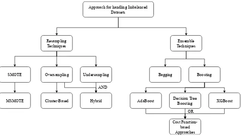
Fig. 1: Approaches for handling skewed distribution of the class
process. This has introduced many interesting problems involving the trade-off required between accuracy and costs. It is clear that, there are existing cost-sensitive AdaBoost algorithms which can solve two-class balanced problems well while other types of prob-lems cause difficulties. Moreover, existing algorithms do not scale for big datasets. In particular, several authors have recognized that there can be a reduction in performance [5] or a trade-off between accuracy and minimizing cost [4]. Along with cost-sensitive learn-ing MapReduce can be used to achieve parallelism so that multiple commodity hardware can be used to process big datasets. In boost-ing based cost-sensitive learnboost-ing the goal is to reduce costs. There-fore, methods such as voting with minimum expected cost criteria from the ensemble of classifiers and incorporating misclassifica-tion cost in the model building phase using weight update rule of all models of the ensemble of classifiers can be used to reduce the cost.
Hence, this research aims to use MapReduce as a basis for devel-oping a cost-sensitive boosting algorithm and aims to address the trade-off between cost and accuracy, that has been observed in pre-vious studies.
The following section presents the background on handling skewed distribution of classes and cost-sensitive boosting. Existing re-search gaps are discussed in section 3 along with the contribution of this research. Distributed Decision Tree (DDT) and DDTv2 are ex-plained in section 4.1 and 4.2 respectively. Then, working of CsDb algorithm is explained in section 5 followed by its empirical evalu-ation (section 5.1). Results and discussion follows in in section 5.2. Finally, section 6 summarizes the this paper and presents future di-rections.
2. BACKGROUND
2.1 Approaches for handling skewed distribution of the class
Class imbalance problem is also known as the skewed distribution of classes problem. This happens, typically, when the number of instances of one class (For example, positive) is far less than the number of instances of another class (For example, negative). This problem is extremely common in practice and can be observed in various disciplines including fraud detection, anomaly detection, medical diagnosis, facial recognition, clickstream analytics, etc. Due to the prevalence of this problem, there are many approaches to deal with it. In general, these approaches can be classified into two major categories - 1) Data level approach - resampling techniques, and 2) Algorithmic ensemble techniques as shown in Figure 1. Re-sampling techniques can be broken into three major categories: a)
Oversampling, b) Undersampling, and c) Synthetic Minority Over-sampling Technique (SMOT). The algorithmic techniques can be divided into two major categories: a) Bagging, and b) Boosting.
2.2 Cost-sensitive Boosting
Data mining classification algorithms can be classified into two cat-egories, namely, error based model (EBM) and cost based model (CBM). EBM does not incorporate the cost of misclassification in the model building phase while CBM does. EBM treats all errors as equally likely but this is not the case with all real world applica-tions - credit card fraud detection systems, loan approval systems, medical diagnosis, etc., are some examples where the cost of classifying one class is usually much higher than the cost of mis-classifying the other class.
Boosting and bagging approaches reduce variance and provide higher stability to a model. Boosting, however, tries to reduce bias (overcomes under fitting) whereas bagging tries to solve the high variance (over fitting) problem. Datasets with skewed class distri-butions are prone to high bias. Therefore, it is natural to choose boosting over bagging to solve the class imbalance problem [4]. The intuition behind cost (function) based approaches is that, in the case of a false negative being costlier than a false positive, one false negative is over counted as, say, n false negatives, wheren >1. For example, if a false negative is costlier than a false positive, the ma-chine learning algorithm tries to make fewer false negatives com-pared to false positives (since it is cheaper). Penalized classification imposes an additional cost on the model for making classification mistakes on the negative class during training. These penalties can bias the model to pay more attention to the negative class. Boosting involves creating a number of hypothesesht and com-bining them to form a more accurate, composite hypothesis of the form
f(x) =
T
X
t=1
αtht(x) (1)
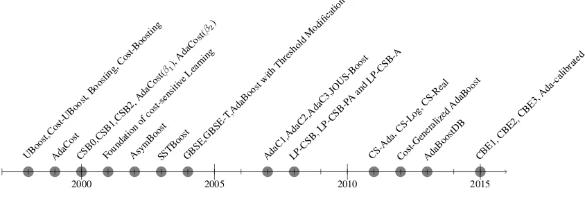
whereαtindicates the extent of the weight that should be given toht(x). In AdaBoost for instance, initial weights arem1 for each sample. It is important to note that these weights are increased us-ing a weight update equation if a sample is misclassified. Weights are decreased if a sample is classified correctly. At the end, hypoth-esishtis available which can be combined to perform classifica-tion. In summary, AdaBoost can be considered to be a three-step process, that is, initialization, weight update equations, and a final weighted combination of the hypotheses. All Cost-sensitive (CS) Boosters (Figure 2) are adaptations of the three step process of Ad-aBoost to design cost-sensitive algorithms.
3. EXISTING RESEARCH GAPS
2000 2005 2010 2015 UBoost,Cost-UBoost,
Boosting, Cost-Boosting
AdaCost Foundation ofcost-sensiti
veLearning
CSB0,CSB1,CSB2, AdaCost(
β1),
AdaCost( β2)
AsymBoostSSTBoostGBSE,GBSE-T ,AdaBoost
with Threshold
Modification
AdaC1,AdaC2,AdaC3,JOUS-BoostLP-CSB, LP-CSB-P
Aand LP-CSB-A
CS-Ada, CS-Log,
CS-Real
Cost-Generalized AdaBoost
AdaBoostDB CBE1, CBE2,
[image:3.595.91.513.73.215.2]CBE3, Ada-calibrated
Fig. 2: Timeline of CS Boosters
gigabytes or beyond fuels an interesting debate - to which DDM re-searchers should pay attention. Nevertheless, faster data mining is necessary. Easy decomposability of data mining algorithms makes them ideal candidates for parallel processing. This can be achieved using a distributed data mining system.
Class imbalance problem can be handled by approaches discussed in section 2.1. The algorithmic ensemble techniques are suitable candidates for scaling to datasets of volumes beyond gigabytes. Some real world problems, however, come with data sizes in gi-gabytes or terabytes for training with biased class distribution. For example, click stream data [20]. Therefore, there is a need to de-sign an algorithm of machine learning which can learn from these datasets. In this case, DDM can provide an effective solution. In earlier work [17, 18] cost-based approach was used to address the class imbalance problem, using data mining as explained in the next paragraph. Most of the solutions as discussed in Section 2.1 for solving the class imbalance problem do not scale to the vol-ume of data beyond the capacity of commodity hardware to han-dle. Therefore, there exists a need to modify CSE1-5 [17] so that it can address the said challenge. Moreover, it is important to pre-serve accuracy, precision, recall, F-measure, number of high-cost errors, and misclassification cost of a DDM based implementation of an algorithm with respect to its stand alone implementation. For fast iterations of data mining modelling, the model building time should be reduced. The choice of these performance measures is explained in section 5.1.
In a distributed system, many commodity machines are connected together to do a single task in an efficient way. In distributed data mining processes, many commodity hardware work together to ex-tract the knowledge from the data stored across all the nodes. The data analytics approaches can be divided into three categories de-pending upon the volume of the data they consider. The first ap-proach is based onmachine learning and statistics. Here, if data can be read from a disk into the main memory, the algorithm runs and reads the data available in the main memory. This leads to a sit-uation where repetitive disk access is needed. Such an architecture is a single node architecture. The second approach is as follows. If data does not fit into the main memory aclassical data mining1the algorithm looks into the disk in addition to looking into the mem-ory. This is calleddata mining[6, 7]. Only a portion of the data is brought into memory at a time. The algorithm processes the data
1It is the computational process of discovering patterns in large data sets involving
methods at the intersection of artificial intelligence, machine learning, and statistics.
in parts and writes back partial results to the disk. Sometimes even this is not sufficient as in the case of Google crawling web pages. This requires the third approach, that is, distributed environment [9, 14, 12, 13, 10, 11, 15, 16].
As discussed in this section there is a need for a fast, distributed, scalable, and cost-sensitive data mining algorithm.
4. DISTRIBUTED DECISION TREE
4.1 Distributed Decision Tree (DDT) and Spark Tree (ST)
Using standalone commodity hardware with limited gigabytes of primary memory and only tens of cores, mining gigabytes of data is not possible using machine learning and statistics whereas it can take hours or days to generate a model using classical data min-ing algorithms (section 3). Therefore, as described in section 3 the third approach is used in the implementation of DDT and Spark Trees (ST). DDT or ST could be used when a dataset is not accom-modatable in memory or processing would take hours or days on a single machine. The task is to build decision tree from dataset of size gigabytes and beyond with hundreds of attributes. The goal is to have a tree which can fit in memory. MapReduce is used to achieve the same. DDT and ST are suited to offline batch-based processing of datasets of size beyond the capacity of commodity hardware to handle it. The algorithm works on an idea of the divide (data) and conquer over multiple processing machines.
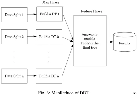
The approach of DDT and ST is as follows. As defined in Figure 3, before the MapReduce phase, the dataset is divided into a number of splits defined by the user. In the next step, that is, Map, it creates decision trees using chunks of data available on each data node. In the reduce step, it collects all the models created in the map tasks. Basically, in the case when decision tree is considered as a base classifier, an ensemble of trees is generated. In general, in the case of non-aggregatable classifiers (for example, decision tree), the final model produced from the reducer is a voted ensemble of the models learned by the mappers [19].
Fig. 3: MapReduce of DDT
This whole mechanism leads to the following problems. First, the Model Experience Problem. If the user supplies hundred partitions as an input, there will be an ensemble of hundred trees after train-ing. In this case, the amount of time required to generate a model will be low but the accuracy will also be low. This case is analogous to consulting a hundred doctors with bachelor of medicine degrees and taking their opinions for a probable diagnosis and concluding that the diagnosis is the one with the maximum votes. Second, the Trade-off Problem. The trade-off is between the size of each parti-tion and accuracy. Consider a case where the size of each partiparti-tion is considerably small. Either because the dataset is small or the number of partitions are large or both. In such cases, trees gener-ated out of each partition would have learnt from a small number of samples. Therefore, its predictive accuracy will be low. If the con-verse is considered, that is, if the size of each partition is very large (either because of a large dataset or a small number of partitions or both) the partitions will not fit into the primary memory (or the pri-mary memory needs to be increased). Of course, if the dataset can fit into the memory and if training is possible, the accuracy of pre-diction will be high, as the learning would take place from a large number of samples.
4.2 Distributed Decision Tree v.2.0
The way DDTv2 and DDT work are similar except in dataset split step, that is,hold the modelapproach is considered in DDTv2. In “Hold the model” approach the model prepared by split 1 of the dataset is held aside until it is also trained from split 2 (Figure 4). Therefore, the number of decision trees generated out of DDTv2 is equal to half of the number of splits.
number of models=bn/2c,where, n is number of partitions (2) This strategy of hold the model work to solve two major problems associated with DDT. First, the number of trees will not be equal to the number of partitions. It is possible to apply the “hold the model” strategy up to the last partition but in that case, parallelism will not be achieved everything will be run by single core and ulti-mately learning process will be slow and sequential. By making the number of models equals the number of partitions divided by two parallelisms is not lost and at the same time, each decision tree will be trained on the double number of samples (note: each partition is of equal size). This is analogous to consulting 50 more experi-enced bachelor of medicine doctors in place of 100 and final dis-ease is concluded as a maximum of 50 votes. Second, the trade-off between the size of partition and accuracy. DDTv2 will
[image:4.595.63.300.72.234.2]accommo-Fig. 4: MapReduce of DDTv2
Table 1. : % Reduction of sot and nol in DDT, ST and DDTv2 with respect to BT and DT
DDT ST DDTv2
BT DT BT DT BT DT
sot 82% 71% 67% 48% 64% 44%
nol 81% 70% 65% 45% 61% 38%
date as large datasets as DDT in memory due to an equal number of partition but will improve on accuracy because each tree will now learn from two partitions in oppose to one in DDT. So consider the case, size of the partition to be smaller (hundreds of samples or in kilobytes) then also it is guaranteed to learn from double the samples. On the other end, if the reverse case is considered, i.e. number of partition is too many (more than 10x for megabytes of data) then there will be a chance to double the number of partitions such that it can accommodate each partition in memory without worrying about generating many trees and compromise in accuracy by avoiding many small partitions.
The DDT, ST and DDTv2 were empirically evaluated over ten selected datasets from UCI machine learning repository and one click-stream dataset from Yahoo! (further details about the dataset is mentioned in section 5.1). The decision tree, ensemble of trees using boosting (BT), DDT, ST, and DDTv2 are compared over three parameters namely, accuracy, size of tree (sot) and number of leaves (nol) of tree(s). Average accuracy of DT, BT, DDT, ST and DDTv2 over all ten selected datasets are 92.79, 99.70, 83.76, 86.93, 97.16, respectively. Even with large dataset DDTv2 is proved to produce accurate results with an acceptable learning time. Dis-tributed implementations of decision tree (DDT, ST and DDTv2) outperformed DT and BT in terms of size of tree and number of leaves with acceptable accuracy of classification. Table 1 shows percentage reduction obtained in size of tree and number of leaves in DDT, ST and DDTv2 with respect to BT and DT.
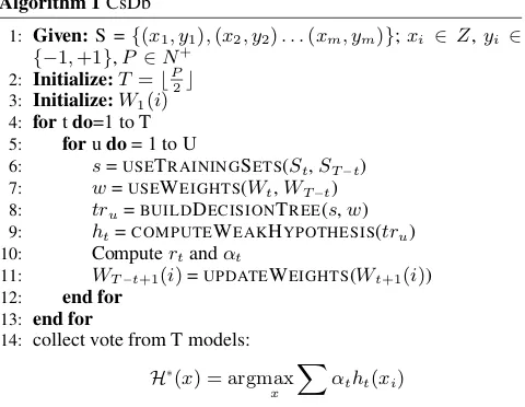
5. COST-SENSITIVE DISTRIBUTED BOOSTING The distributed nature of DDTv2 [20] and cost sensitivity of CSE1-5 [17] are derived into CsDb. CsDb is designed as a meta classifier so that, it can use a weak learner (for decision tree, ibk, etc) as a base classifier. A generalized wrapper which works in replacement for CSExtensions is depicted in algorithm 1.
[image:4.595.326.561.80.223.2]Algorithm 1CsDb
1: Given:S ={(x1, y1),(x2, y2). . .(xm, ym)};xi ∈ Z,yi ∈
{−1,+1},P∈N+ 2: Initialize:T =bP
2c 3: Initialize:W1(i) 4: fortdo=1 to T 5: forudo= 1 to U
6: s=USETRAININGSETS(St,ST−t)
7: w=USEWEIGHTS(Wt,WT−t)
8: tru=BUILDDECISIONTREE(s,w) 9: ht=COMPUTEWEAKHYPOTHESIS(tru) 10: Computertandαt
11: WT−t+1(i)=UPDATEWEIGHTS(Wt+1(i)) 12: end for
13: end for
14: collect vote from T models:
H∗
(x) = argmax
x
X
αtht(xi)
Table 2. : Characteristics of selected datasets
data-set #c #i #n #no group skewness
echo 2 132 11 2
group-1
31.82
sonar 2 208 60 1 3.37
bupa 2 345 6 1 7.97
hv-84 2 435 12 5 11.38
crx 2 690 6 10 5.51
bcw 2 699 6 1 15.52
pima 2 768 8 1 15.10
hypo 2 3163 7 19
group-2 45.23
krkp 2 3196 33 4 2.22
Yahoo! 2 1M 9 1
group-3 46.83
IQM 2 1B 7 6 45.22
Note: #c = number of Classes, #i = number of Instances, #n = number of Numeric attributes and #no = number of NOminal attributes
user. During the map phase, it trains a weak learner (decision tree is used as a weak learner) using distributionWt and WT−t and training setStandST−t. Next, it computes weak hypothesisht : Z→R. Thereafter, by computingrtandαtit also updates weights Wt+1(i)toWT−t+1(i)as per rules defined in CSEx. Finally, in the reducer, it collects the vote from T models using
H∗
(x) = argmax
x
X
αtht(xi)
5.1 Experimental setups
Weka is a collection of open source machine learning algorithms. DDTv2 was implemented as an extension of Weka. The CsDb is implemented as an extension of DDTv2 [20] and CSE1-5 [17]. To test the performance of CsDb, nine datasets, namely, breast cancer Wisconsin (bcw), liver disorder (bupa), credit screening (crx), echocardiogram (echo), house-voting 84 (hv-84), hypothy-roid (hypo), king-rook versus king-pawn (krkp), pima indian dia-betes (pima), and sonar (sonar) from UCI machine learning repos-itory were selected. These datasets belong to various domains. In addition, an algorithm is evaluated using Yahoo! webscope dataset [21] and IQM bid log dataset. Here, IQM bid log dataset is the pro-prietary dataset of IQM Co. It is not available in the public domain. The skewness of the data which is explained in the next paragraph is the reason for selecting these datasets. The datasets are
prepro-cessed to meet the need for classification. For example, the class la-bels were 1 and 0 in the original dataset. They were replaced by ‘y’ and ‘n’ respectively. In Yahoo! webscope dataset attributes other than class label are numeric values of user and article characteris-tics. The sample records with class labels are as under.
UF2, UF3, UF4, UF5, UF6, AF2, AF3, AF4, AF5, AF6, class 0.013, 0.01, 0.04, 0.023, 0.97, 0.21, 0.067, 0.045, 0.23, 0.456, y 0.096, 0.0032, 0.481, 0.112, 0.004, 0.127, 0.0002, 0.0325, 0.123, 0.234, n
In the case of the IQM dataset the fields of interest are encoded for the purpose of privacy. Its sample records are as under. Here, for a given bid request, whether the user clicks on advertise (creative) or not is considered a classification problem.
attrib1, attrb2, attrib3, attrib4, attrib5, attrib6, attrib7, attrib8, attrib9, at-trib10, class, attrib12, attrib13
12, type3, man2, db3, ba, 2.3, 2.5, 430, 120, type3, n, 0, 54321 31, type2, man1, db4, dc, 0.7, 0.4, 620, 120, type1, y, 1, 98765
[image:5.595.54.294.72.258.2]According to the number of instances (#i) as listed in table 2. the datasets are grouped into three categories for the purpose of re-sult analysis. The first group contains echo, sonar, bupa, hv-84, crx, bcw, and pima datasets. They have a few hundred instances (#i∈[100,999]). The second group contains hypo and krkp. The second group can contain datasets with the number of instances [1000, 99999]. The last group contains Yahoo! and IQM datasets with a million and a billion instances respectively. The third group can contain datasets with more than 99,999 instances. An instance in any group can have a size of [1, 10] kilobytes. The skewness in table 2 represents the distribution of the number of instances of mi-nority class over majority class. Here, the skewness index can take any value between0and50where0means no skewness and50 means the highest possible skewness. Average skewness of datasets in group-1, 2 and 3 is 12.95%, 23.72%, and 46.02% respectively. The important characteristics of datasets are summarized in table 2.
The key measure to evaluate the performance of the algorithms for cost-sensitive classification is the total cost of misclassification made by a classifier (That is,P
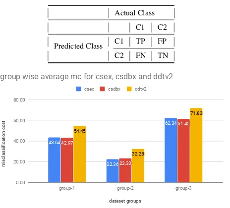
m= cost(actual(m), predicted(m))) [18]. In addition, the number of high cost errors is also used. It is the number of misclassifications associated with max(false-positive, false-negative) in cost matrix to that of in confusion matrix. The model building time is the amount of time taken to build a model. Other than these, accuracy, precision, recall, and F-measure, are used to evaluate the performance of the algorithm. To define these measures TP (true positive), TN (true negative), FP (false positive) and FN (false negative) terms are used. These terms are derived from the confusion matrix. The structure of confusion matrix for binary class problem is shown in Table 3. In Table 3 C1 and C2 are defined as class-1 and class-2 respectively. Now, the accuracy is defined asaccuracy=(T P+(T NT P++T NF P+)F N), and hence the accu-racy defines how well a binary classification test correctly identifies a condition. Precision is defined asprecision= T P
(T P+F P). Preci-sion can be interpreted as a ratio of all events the classifier predicted correctly to all the events the classifier predicted, correctly or incor-rectly. Recall is defined asrecall= (T PT P+F N). Therefore, recall is the ratio of the number of events a classifier can correctly recall to the number of all correct events. F-measure, which is also known as F1-score, is the harmonic mean of precision and recall. Therefore, F−measure= 2∗ precision∗recall
precision+recall.
Table 3. : A confusion matrix structure for a binary classifier Actual Class
C1 C2
Predicted Class C1 TP FP
C2 FN TN
43.64
22.36
62.34
42.97
23.33
61.45
54.45
32.25
71.83
dataset groups
misclassification cost
0.00 20.00 40.00 60.00 80.00
group-1 group-2 group-3 csex csdbx ddtv2
group wise average mc for csex, csdbx and ddtv2
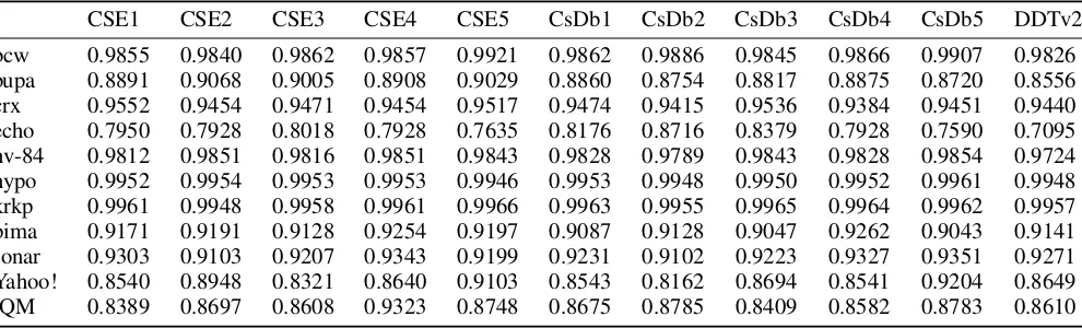
Fig. 5: Group wise average mc for csex, csdbx and ddtv2 11∗6)runs were performed.
The CsDb is a meta-classifier and for this experimental setup, Weka’s implementation of decision tree with default parameter set-tings is used as a weak learner.
The experiments of the CsDb and DDTv2 were performed using Elastic MapReduce (EMR) cluster of Amazon. The EMR for these experiments was configured with one master (c4.4xlarge) and three slaves (c4.4xlarge) nodes. A single instance of c4.4xlarge comes with 16 vCPUs and 30 GiB of memory. To run CSE an r4.8xlarge instance of Amazon Elastic Compute Cloud (Amazon EC2) was used. An r4 series instance r4.8xlarge features 32 vCPUs, 244 GiB of memory.
5.2 Results and Discussion
The algorithm is analysed empirically in this section. Parameter wise, the comparison is broken down into sub-sections. As the mis-classification cost and the number of high cost errors are cost-based parameters they are discussed together in section5.2.1. Secondly, the accuracy, precision, recall, and F-measure are discussed to-gether as they are similar in nature (section5.2.2). Lastly, in section 5.2.3the algorithms are compared for the time they take to build the model. For each parameter, the dataset group wise analysis was performed. The dataset groups are defined in table 2 and discussed in section 5.1.
5.2.1 Misclassification cost and number of high-cost errors. CsDb when compared with CSE over group 1, 2, and 3 datasets the misclassification cost varies, on an average, by 2.44% (for group-1, 2 and 3 it is 1.54%, -4.35% and 1.43% respectively) and the number of high cost errors by 14.30% (for group-1, 2 and 3 it is 5.52%, -31.59% and -5.79% respectively). CsDb produces 21.06% (for group-1, 2 and 3 it is 21.08%, 27.65% and 14.45% respec-tively) fewer misclassification errors and 30.15% (for group-1, 2 and 3 it is 31.39%, 27.11% and 31.94% respectively) less number of high cost errors when compared with DDTv2.
These results indicate CsDb can preserve cost sensitivity of CSE. DDTv2 produces an average number of high cost errors of 5.64 and average misclassification cost of 54.45 over all the dataset groups. This is natural because DDTv2 is a classifier of EBM category. It is
4.10
2.08
3.86 3.87
2.73
4.08
5.64
3.75
6.00
dataset groups
# HCE
0.00 2.00 4.00 6.00
group-1 group-2 group-3 csex csdbx ddtv2
group wise average # hce for csex, csdbx and ddtv2
[image:6.595.61.293.79.289.2]Fig. 6: Group wise average number of hce for csex, csdbx and ddtv2 important to note here that pima dataset in group-1 produces 35% more misclassification cost and the number of high cost errors with respect to its group-1 average. This is due to the numerical ranges of numerical features in the dataset. After feature scaling (feature normalization) it was observed that this error was reduced to 20%. Figure 5 and 6 show group wise average misclassification cost and number of high cost errors respectively. Table 4 shows average mis-classification cost (mc) and number of high cost error (#hce) over the selected cost matrix for CSE1-5, CsDb1-5 and DDTv2.
5.2.2 Accuracy, precision, recall, and F-measure. Analysing CsDb when compared with CSE over group 1, 2, and 3 datasets the average accuracy variation is 1% (for group1, 2 and 3 it is 0.01%, -0.02% and 1.26%, respectively) whereas comparing it with DDTv2 average improvement of 2.15% (for group-1, 2 and 3 it is 2.21%, 0.05% and 4.20%, respectively) is observed.
In group 3 data, average accuracy is 5% less than the mean accuracy across all datasets. It is possible because skew factor in group 3 datasets is 45 (table 2) that is, 90% of its maximum possible value. It is important to note that group 1 dataset echo shows accuracy below 80% . This is mainly because it has just 132 instances and its numerical features are not normalized. After normalization, an accuracy improvement of 2.76% was observed in echo.
Table 5 shows average accuracy over the selected cost matrix for CSE1-5, CsDb1-5 and DDTv2.
Precision, recall, and F-measure for CsDb with respect to CSE over the datasets of group 1, 2 and 3 varies on average by 1% (for group-1, 2 and 3 it is 0.62%, 0.47% and 0.47%, respectively), 1.44% (for group-1, 2 and 3 it is 0.39%, 0.50% and 3.44%, respectively), and 0.97% (for group-1, 2 and 3 it is 0.16%, 0.04%, and 2.71%, re-spectively). When compared to DDTv2 precision and recall varies on an average by 1.71% (for group-1, 2, and 3 it is 2.43%, 0.74% and 1.97%, respectively), 1.89% (for group-1, 2 and 3 it is 1.53%, 1.14% and 3.01%, respectively), and 2.77% (for group 1, 2 and 3 it is 2.19%, 0.21% and 5.92%, respectively).
This is because CsDb is CBM and boosting technique and hence it can maintain bias variance trade-off and hence able to balance pre-cision and recall. Hence, F-measure is also balanced within 1.5%. Moreover, DDTv2 is EBM based and hence fails to balance be-tween precision and recall. Hence, F-measure is also increased by 8.73%.
Table 6 shows average precision, recall and F-measure over the se-lected cost matrix for CSE1-5, CsDb1-5 and DDTv2.
Table 4. : Misclassification cost and Number of High cost errors of CSE1-5, CsDb1-5, DDTv2 (mc / #hce)
[image:7.595.60.555.208.358.2]CSE1 CSE2 CSE3 CSE4 CSE5 CsDb1 CsDb2 CsDb3 CsDb4 CsDb5 DDTv2 bcw 14.69 / 1.00 15.82 / 1.00 14.57 / 1.00 15.67 / 1.50 12.67 / 1.33 14.67 / 1.67 19.33 / 2.50 15.17 / 1.50 14.00 / 1.50 13.67 / 2.17 33.00 / 4.33 bupa 59.71 / 5.74 60.32 / 5.47 58.79 / 5.61 57.33 / 4.17 59.67 / 6.00 58.83 / 4.17 59.83 / 4.50 61.33 / 3.67 58.50 / 3.50 61.00 / 3.33 68.67 / 4.50 crx 59.55 / 7.04 60.83 / 5.31 59.33 / 5.30 56.83 / 5.50 59.50 / 5.50 60.33 / 5.50 58.67 / 4.33 55.83 / 5.83 57.17 / 5.83 59.00 / 5.00 68.50 / 7.00 echo 22.63 / 2.31 24.52 / 2.51 24.27 / 2.13 26.33 / 3.50 29.00 / 3.17 20.83 / 2.33 17.00 / 2.33 21.83 / 1.67 26.83 / 2.67 25.50 / 2.17 34.67 / 3.83 h-d 36.65 / 4.20 34.74 / 3.06 35.46 / 3.61 37.83 / 5.17 37.50 / 3.67 32.83 / 3.33 38.33 / 3.83 35.50 / 5.83 38.67 / 4.17 37.00 / 4.67 50.00 / 6.17 hv-84 11.43 / 0.95 10.61 / 0.69 12.45 / 0.81 12.00 / 1.33 10.83 / 1.17 10.17 / 0.83 11.83 / 0.83 11.83 / 1.33 12.50 / 1.33 11.83 / 1.50 25.17 / 3.33 hypo 25.24 / 2.50 24.58 / 2.52 26.59 / 2.57 24.17 / 2.67 25.17 / 1.67 28.33 / 4.17 29.33 / 2.83 26.33 / 3.33 24.67 / 2.67 26.67 / 4.50 35.00 / 4.50 krkp 19.20 / 1.55 21.42 / 1.27 19.41 / 1.36 18.83 / 2.17 19.00 / 2.50 17.67 / 1.50 21.67 / 2.50 20.00 / 2.33 17.17 / 1.50 21.50 / 2.00 29.50 / 3.00 pima 111.69 / 10.39 113.16 / 10.81 110.79 / 10.38 112.17 / 12.50 113.83 / 11.50 112.33 / 12.33 113.33 / 11.83 111.67 / 10.67 111.00 / 11.67 113.83 / 10.33 121.83 / 12.83 sonar 23.18 / 1.93 23.25 / 1.10 23.46 / 1.60 23.33 / 1.83 23.33 / 1.33 19.67 / 1.00 22.00 / 1.00 21.17 / 0.83 21.83 / 1.83 19.67 / 2.00 29.33 / 3.67 Yahoo! 76.03 / 2.76 80.15 / 1.63 75.48 / 1.61 70.00 / 3.17 76.00 / 2.17 74.33 / 2.50 77.00 / 2.50 75.00 / 2.83 74.00 / 1.50 74.83 / 3.33 85.00 / 5.67 IQM 47.68 / 5.28 50.23 / 5.52 49.34 / 4.97 50.33 / 6.33 48.17 / 5.17 49.67 / 6.00 48.17 / 5.33 44.83 / 5.00 47.83 / 5.33 48.83 / 6.50 58.67 / 6.33
Table 5. : Accuracy of CSE1-5, CsDb1-5, DDTv2
CSE1
CSE2
CSE3
CSE4
CSE5
CsDb1
CsDb2
CsDb3
CsDb4
CsDb5
DDTv2
bcw
0.9855
0.9840
0.9862
0.9857
0.9921
0.9862
0.9886
0.9845
0.9866
0.9907
0.9826
bupa
0.8891
0.9068
0.9005
0.8908
0.9029
0.8860
0.8754
0.8817
0.8875
0.8720
0.8556
crx
0.9552
0.9454
0.9471
0.9454
0.9517
0.9474
0.9415
0.9536
0.9384
0.9451
0.9440
echo
0.7950
0.7928
0.8018
0.7928
0.7635
0.8176
0.8716
0.8379
0.7928
0.7590
0.7095
hv-84
0.9812
0.9851
0.9816
0.9851
0.9843
0.9828
0.9789
0.9843
0.9828
0.9854
0.9724
hypo
0.9952
0.9954
0.9953
0.9953
0.9946
0.9953
0.9948
0.9950
0.9952
0.9961
0.9948
krkp
0.9961
0.9948
0.9958
0.9961
0.9966
0.9963
0.9955
0.9965
0.9964
0.9962
0.9957
pima
0.9171
0.9191
0.9128
0.9254
0.9197
0.9087
0.9128
0.9047
0.9262
0.9043
0.9141
sonar
0.9303
0.9103
0.9207
0.9343
0.9199
0.9231
0.9102
0.9223
0.9327
0.9351
0.9271
Yahoo!
0.8540
0.8948
0.8321
0.8640
0.9103
0.8543
0.8162
0.8694
0.8541
0.9204
0.8649
IQM
0.8389
0.8697
0.8608
0.9323
0.8748
0.8675
0.8785
0.8409
0.8582
0.8783
0.8610
sensitivity and other efficiency measures. However, over group 1 and group 2 datasets, the difference between model building time of CSE and CsDb is 2% on average.
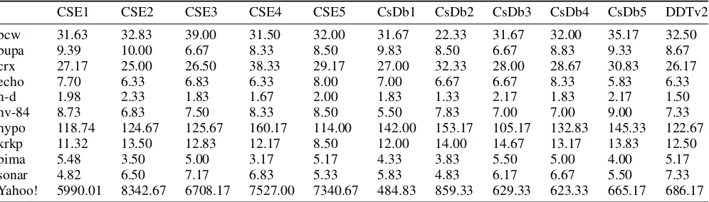
Table 7 shows average model building times over the selected cost matrix for CSE1-5, CsDb1-5 and DDTv2.
6. CONCLUSION
The goal of this research work is to improve CBM for the volume of data which cannot be handled by standalone commodity hardware. The work reviewed various alternatives to handling the class im-balance problem. The results show variation in accuracy, misclas-sification cost and high cost errors by 1%, 2%, and 7% respectively when CsDb is compared to CSE. This proves that CsDb is able to preserve the cost-sensitivity of CSE. Whereas, the cost-sensitivity is improved drastically when compared with a error based classi-fier.
As described in section 5 advantages of CSE1-5 and DDTv2 are combined in CsDb. The CsDb is a fast, distributed, scalable, and cost-sensitive implementation of type CBM algorithm. It follows the boosting technique and helps overcome the class imbalance problem. Section 5.2 shows how the misclassification cost and the number of high cost errors in CsDb varies by just 2% and 14% respectively when compared to CSE and improves by 21.06% and 30.15% respectively when compared with DDTv2. Moreover, model building time is improved by 90%. Finally, the average vari-ation in F-measure between CSE and CsDb is just 0.97%. Moreover, the DDTv2 which is a distributed version of the decision tree implementation and works on the ‘hold the model’ concept and when compared with BT and DT (section 4.2), outperforms them in terms of accuracy, size of tree, and number of leaves. Using DDTv2, the size of the tree is reduced by 64% and 44% compared
with BT and DT, respectively. Whereas, the number of leaves is reduced by 61% and 38%, respectively. All this is achieved without compromising on classification accuracy. Moreover, the DDTv2 is able to reduce model building time by 15% as it builds the tree in a distributed way. DDTv2 works to solve two major problems, namely, model experience and trade-off between size of partition and performance associated with DDT.
The three verticals have been identified in which this research can be extended. First, the performance of CsDb is dependent upon the choice of weak learner. One can use different weak learners (For example, Decision Stump) to compare the results with re-spect to decision tree. Coming up with a strategic way of choos-ing a weak learner to improve performance of CsDb is an impor-tant future extension. Second, recently, there has been significant amount of research work in automated hyperparameters tuning of a classification algorithm. CsDb has sensitive hyperparameters such as cost-matrix. Automatic tuning of the hyperparameters of CsDb using neural networks is an important research extension. Lastly, as shown in Figure 1 there exist multiple methods for handling skewed distribution of the class. An empirical comparison between CsDb and other approaches for handling skewed distribution of class can provide concrete conclusions on a vertical of scalability of the methods.
7. REFERENCES
[1] Elkan, C. (2001). The foundations of cost-sensitive learning. In International joint conference on artificial intelligence Vol. 17, No. 1, pp. 973-978.
Table 6. : Precision, Recall and F-measure of CSE1-5, CsDb1-5, DDTv2 (precision / recall / f-measure)
CSE1 CSE2 CSE3 CSE4 CSE5 CsDb1 CsDb2 CsDb3 CsDb4 CsDb5 DDTv2
bcw 0.99 / 0.99 / 0.99 0.99 / 0.99 / 0.99 0.99 / 0.99 / 0.99 0.99 / 0.99 / 0.99 0.99 / 1.00 / 0.99 0.99 / 0.99 / 0.99 0.99 / 0.99 / 0.99 0.99 / 0.99 / 0.99 0.99 / 0.99 / 0.99 0.99 / 0.99 / 0.99 0.99 / 0.99 / 0.99 bupa 0.83 / 0.86 / 0.84 0.90 / 0.90 / 0.89 0.89 / 0.89 / 0.88 0.87 / 0.89 / 0.87 0.88 / 0.90 / 0.88 0.87 / 0.88 / 0.86 0.82 / 0.90 / 0.84 0.88 / 0.87 / 0.86 0.87 / 0.89 / 0.86 0.85 / 0.87 / 0.84 0.82 / 0.86 / 0.82 crx 0.95 / 0.95 / 0.95 0.94 / 0.94 / 0.94 0.94 / 0.95 / 0.94 0.94 / 0.94 / 0.94 0.94 / 0.96 / 0.95 0.93 / 0.95 / 0.94 0.94 / 0.93 / 0.93 0.95 / 0.95 / 0.95 0.92 / 0.95 / 0.93 0.95 / 0.94 / 0.94 0.93 / 0.94 / 0.94 echo 0.91 / 0.83 / 0.86 0.85 / 0.87 / 0.85 0.85 / 0.88 / 0.84 0.85 / 0.87 / 0.85 0.85 / 0.83 / 0.83 0.86 / 0.88 / 0.86 0.91 / 0.91 / 0.91 0.88 / 0.90 / 0.88 0.80 / 0.90 / 0.83 0.78 / 0.87 / 0.80 0.75 / 0.82 / 0.76 hv-84 0.98 / 0.97 / 0.98 0.98 / 0.98 / 0.98 0.98 / 0.97 / 0.98 0.98 / 1.00 / 0.98 0.98 / 0.98 / 0.98 0.98 / 0.98 / 0.98 0.98 / 0.97 / 0.97 0.98 / 0.98 / 0.98 0.97 / 0.98 / 0.98 0.98 / 0.98 / 0.98 0.96 / 0.97 / 0.96 hypo 0.95 / 0.95 / 0.95 0.98 / 0.93 / 0.95 0.97 / 0.94 / 0.95 0.95 / 0.96 / 0.95 0.94 / 0.95 / 0.94 0.93 / 0.97 / 0.95 0.94 / 0.95 / 0.94 0.93 / 0.96 / 0.95 0.98 / 0.93 / 0.95 0.95 / 0.97 / 0.96 0.96 / 0.93 / 0.95 krkp 1.00 / 1.00 / 1.00 0.99 / 1.00 / 1.00 1.00 / 1.00 / 1.00 0.99 / 1.00 / 1.00 1.00 / 1.00 / 1.00 1.00 / 1.00 / 1.00 1.00 / 1.00 / 1.00 1.00 / 1.00 / 1.00 1.00 / 1.00 / 1.00 1.00 / 1.00 / 1.00 1.00 / 1.00 / 1.00 pima 0.94 / 0.94 / 0.94 0.94 / 0.94 / 0.93 0.94 / 0.93 / 0.93 0.94 / 0.95 / 0.94 0.94 / 0.94 / 0.94 0.93 / 0.93 / 0.93 0.92 / 0.94 / 0.93 0.94 / 0.92 / 0.93 0.94 / 0.95 / 0.94 0.93 / 0.93 / 0.93 0.93 / 0.94 / 0.93 sonar 0.91 / 0.95 / 0.92 0.90 / 0.92 / 0.90 0.92 / 0.92 / 0.92 0.92 / 0.94 / 0.93 0.91 / 0.93 / 0.91 0.92 / 0.93 / 0.92 0.88 / 0.94 / 0.90 0.92 / 0.93 / 0.92 0.90 / 0.95 / 0.92 0.95 / 0.92 / 0.93 0.91 / 0.93 / 0.92 Yahoo! 0.87 / 0.80 / 0.90 0.90 / 0.87 / 0.88 0.87 / 0.89 / 0.88 0.83 / 0.90 / 0.88 0.84 / 0.83 / 0.91 0.85 / 0.88 / 0.84 0.89 / 0.89 / 0.90 0.84 / 0.89 / 0.89 0.92 / 0.86 / 0.86 0.82 / 0.84 / 0.83 0.85 / 0.90 / 0.91 IQM 0.83 / 0.84 / 0.90 0.85 / 0.88 / 0.91 0.88 / 0.79 / 0.91 0.87 / 0.86 / 0.88 0.90 / 0.87 / 0.87 0.90 / 0.86 / 0.85 0.90 / 0.85 / 0.82 0.88 / 0.85 / 0.86 0.86 / 0.89 / 0.84 0.90 / 0.89 / 0.92 0.88 / 0.84 / 0.85
Table 7. : Model Building Time of CSE1-5, CsDb1-5, DDTv2
CSE1 CSE2 CSE3 CSE4 CSE5 CsDb1 CsDb2 CsDb3 CsDb4 CsDb5 DDTv2
bcw 31.63 32.83 39.00 31.50 32.00 31.67 22.33 31.67 32.00 35.17 32.50
bupa 9.39 10.00 6.67 8.33 8.50 9.83 8.50 6.67 8.83 9.33 8.67
crx 27.17 25.00 26.50 38.33 29.17 27.00 32.33 28.00 28.67 30.83 26.17
echo 7.70 6.33 6.83 6.33 8.00 7.00 6.67 6.67 8.33 5.83 6.33
h-d 1.98 2.33 1.83 1.67 2.00 1.83 1.33 2.17 1.83 2.17 1.50
hv-84 8.73 6.83 7.50 8.33 8.50 5.50 7.83 7.00 7.00 9.00 7.33
hypo 118.74 124.67 125.67 160.17 114.00 142.00 153.17 105.17 132.83 145.33 122.67
krkp 11.32 13.50 12.83 12.17 8.50 12.00 14.00 14.67 13.17 13.83 12.50
pima 5.48 3.50 5.00 3.17 5.17 4.33 3.83 5.50 5.00 4.00 5.17
sonar 4.82 6.50 7.17 6.83 5.33 5.83 4.83 6.17 6.67 5.50 7.33
Yahoo! 5990.01 8342.67 6708.17 7527.00 7340.67 484.83 859.33 629.33 623.33 665.17 686.17
[3] Ting, K. M., & Zheng, Z. (1998). Boosting cost-sensitive trees. In International Conference on Discovery Science (pp. 244-255). Springer, Berlin, Heidelberg.
[4] Susan Lomax and Sunil Vadera. (2013). A survey of cost-sensitive decision tree induction algorithms. ACM Comput. Surv. 45, 2, Article 16.
[5] Ting, K. M. (2000). A comparative study of cost-sensitive boosting algorithms. In Proceedings of the 17th International Conference on Machine Learning (pp. 983–990)
[6] Han, J., Pei, J., & Kamber, M. (2011). Data mining: concepts and techniques. Elsevier.
[7] Witten, I. H., Frank, E., Hall, M. A., & Pal, C. J. (2016). Data Mining: Practical machine learning tools and techniques. Mor-gan Kaufmann.
[8] Berry, M. J., & Linoff, G. (1997). Data mining techniques: for marketing, sales, and customer support. John Wiley & Sons, Inc.
[9] Leskovec, J., Rajaraman, A., & Ullman, J. D. (2014). Mining of massive datasets. Cambridge university press.
[10] Palit, I., & Reddy, C. K. (2012). Scalable and parallel boosting with mapreduce. IEEE Transactions on Knowledge and Data Engineering, 24(10), 1904-1916.
[11] Ye, J., Chow, J. H., Chen, J., & Zheng, Z. (2009). Stochas-tic gradient boosted distributed decision trees. In Proceedings of the 18th ACM conference on Information and knowledge management (pp. 2061-2064). ACM.
[12] Lazarevic, A., & Obradovic, Z. (2002). Boosting algorithms for parallel and distributed learning. Distributed and Parallel Databases, 11(2), 203-229.
[13] Abualkibash, M., ElSayed, A., & Mahmood, A. (2013). Highly Scalable, Parallel and Distributed AdaBoost Algorithm
using Light Weight Threads and Web Services on a Network of Multi-Core Machines. arXiv preprint arXiv:1306.1467. [14] Cooper, J., & Reyzin, L. (2017). Improved algorithms for
dis-tributed boosting. In Communication, Control, and Computing (Allerton), 2017 55th Annual Allerton Conference on (pp. 806-813).
[15] Bowyer, K. W., Hall, L. O., Moore, T., Chawla, N., & Kegelmeyer, W. P. (2000). A parallel decision tree builder for mining very large visualization datasets. In Systems, Man, and Cybernetics, 2000 IEEE International Conference on (Vol. 3, pp. 1888-1893).
[16] Shafer, J., Agrawal, R., & Mehta, M. (1996). SPRINT: A scal-able parallel classi er for data mining. In Proc. 1996 Int. Conf. Very Large Data Bases (pp. 544-555).
[17] Desai, A., & Jadav, P. M. (2012). An empirical evaluation of ad boost extensions for cost-sensitive classification. Inter-national Journal of Computer Applications, 44(13), 34-41. [18] Desai, A., Jadav, K., & Chaudhary, S. (2015). An Empirical
evaluation of CostBoost Extensions for Cost-Sensitive Classi-fication. In Proceedings of the 8th Annual ACM India Confer-ence (pp. 73-77). ACM.
[19] Desai, A., & Chaudhary, S. (2016). Distributed Decision Tree. In Proceedings of the 9th Annual ACM India Conference (pp. 43-50).
[20] Desai, A., & Chaudhary, S. (2017). Distributed decision tree v. 2.0. In Big Data (Big Data), 2017 IEEE International Con-ference on (pp. 929-934).
[image:8.595.58.556.190.332.2]