Breast Cancer Detection using SVM Classifier with Grid Search Technique

Breast Cancer Detection using SVM Classifier with Grid

Search Technique

Vishal Deshwal

Student of BSIT, Stratford University, Noida,

India Campus

Mukta Sharma,

Faculty of Computer Science and Information Technology Stratford University, Noida, India

Campus

ABSTRACT

Medical science is a boon to mankind. The technological advancement has widened the scope of curing and fighting with the diseases. It is essential to diagnose the symptoms and identify the disease timely. It has been observed that breast cancer cases are the most reported cases among women around the world and the second most common cancer overall. According to [1] World Cancer Research Fund International, London has shared that there were over 2 million new cases in 2018. In the year 2012, the BCRF (Breast Cancer Research Foundation) has reported nearly 1.7 million new breast cancer cases [2]. With the help of technology, medical science is trying to predict cancer; which can significantly increase the chances of survival. In this research paper, the authors have illustrated the model to predict breast cancer with Support Vector Machine using Grid search. First Support vector machine model is tested without a grid search. Later, Support vector machine model is tested with grid search. Finally, the comparative analysis was done and based on the result; a new model was built. The new model designed is based on grid search on data before fitting it for prediction, which enhances the outcome.

General Terms

Your general terms must be any term which can be used for general classification of the submitted material such as Pattern Recognition, Security, Algorithms et. al.

Keywords

Machine learning; support vector machine; grid search; cancer prediction

1.

INTRODUCTION

It has been observed that medical sciences have grown enormously with the development of technology. Various simulators have been designed using Virtual Reality to train the practitioner. Biomedical science deals with medicines and information technology. According to (Van Bemmel, 1984) biomedical sciences deals with handling information based on the knowledge and expertise derived from practices in medicine and health care both theoretically and practically. As per (Shortliffe and Blois, 2006) defines it as (Concept-based), the technical domain deals with information, storing and retrieving knowledge and making optimal use for problem solving and decision making.

The Breast cancer prediction is one of the most influential research problems in health care community. The aim of this paper is to classify the tumors on based of features obtained from images into malignant (cancerous) or benign (non-cancerous)[3]. In case the final result depicts the tumor to be malignant; patient can get treatment immediately which will help to cure fast.

It could be malignant which is cancerous or benign which is non-cancerous. In case of malignant cells encircles into

nearby tissues and grows in remote areas of body while benign tumor does not lays out in tissues around or to any other parts of body, unlike cancerous tumors. With Machine Learning models the process of cancer diagnosis can be enhanced drastically.

In this paper the quest is to differentiate the malignant and benign tumors using the given features in Breast Cancer dataset provided in Sklearn.datasets library. There is an extensive work done in development and evaluation of support vector machine models for breast cancer prediction using different techniques like normalization and principal component analysis. This paper depicts the working model with different support vector machine technique called grid search. It also shed light on the results and how they have been enhanced dramatically with the help of grid search. Grid search focuses on finding the right value of two major support vector machine parameters which are regularization parameter C and gamma for which model gives the highest accuracy.

2.

MATERIALS AND METHODS

Dataset: It is set of data arranged together which may or may not be interrelated to each other. For creating SVM classifier for breast cancer the dataset used is from sklearn.datasets library. The resources for this dataset can be found at https://www.openml.org/d/15. Breast Cancer Wisconsin (Original) Data Set. Features are computed from a digitized image of a fine needle aspirate (FNA) of a breast mass. They describe characteristics of the cell nuclei present in the image. The target feature records the prognosis (malignant or benign). [4]

Method:

Model 1: Creating a classifier with SVM without grid search: In machine learning a program is said to learn from experience E with respect to some class of task T and performance measure P, if the performance on tasks in T as measured by P improves with experience E. Experience E, is also called as Data and Task T can be prediction, classification etc. In this article, E is the breast cancer dataset and task T is to create a SVM classifier which can classify the cancer into malignant (cancerous) or benign (non-cancerous) on the basis of features given for each instance.

Process of creating a classifier or learner is divided into four steps:

1. Choose the training experience.

2. Choose the target function. (That has to be learned) 3. Choose how to represent a target function.

classification. Though it is very effective classifier for linear data but it can handle non-linearity by using non-linear basis functions or in particular called kernel function. Support Vector machine has a clever way to prevent over-fitting and can work with relatively larger number of features without requiring too many computation.

Detection of tumors in with SVM is divided into four main stages. First stage involves the understanding and reading the given dataset through different plots. Second stage implicates about split of dataset into two parts training and testing. In third stage prediction is done using the normal SVM model followed by limitation faced in this model and reason for getting false predictions.

Fourth stage includes recreating the model with Grid search technique and to find the regularization parameter C and gamma for which model gives the highest accuracy.

Programming language used is python and application used to run the code is Jupiter notebook.

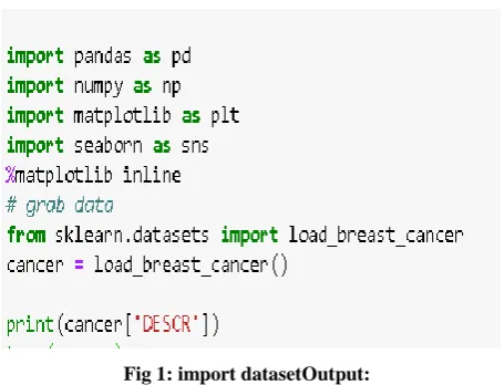
First Stage: Foremost step is to import Dataset.

Fig 1: import datasetOutput:

Breast Cancer Wisconsin (Diagnostic) Database [2]

Data Set Characteristics: Number of Instances: 569, Number of Attributes: 30 numeric, predictive attributes and the class Attribute Information: Radius (mean of distances from center to points on the perimeter), Texture (standard deviation of gray-scale values), Smoothness (local variation in radius lengths), and Compactness (perimeter^2 / area - 1.0), Concavity (severity of concave portions of the contour), Concave points (number of concave portions of the contour), Fractal dimension ("coastline approximation" - 1). The mean, standard error, and "worst" or largest (mean of the three largest values) of these features were computed for each image, Resulting in 30 features. For instance, field 3 is Mean Radius, field 13 is Radius SE, field 23 is Worst Radius. Class: i. WDBC-Malignant, ii. WDBC-Benign Summary of dataset:

There are 569 instances with 30 numeric attributes and prediction which is need to be done is that weather the cancer is malignant (cancerous) or benign (non-cancerous). Now before train-test splitting, it's better to visually analyses the features for this data set for that it has to be converted into data frame. Data frames are 2D data structure in which different columns may have different data types. For visualizing the dataset it is recommended to convert it into

Data frames. There are many prebuilt libraries for visualizing supporting Data frames.

Fig 2: Setting Data frame

It is always better to know correlations between features and target class before applying any model to dataset because it makes it easier to know that either the features is useful or can be removed from dataset. Correlation can be calculated and visualized using seaborn library.

Seaborn is a statistical plotting library built on top of matplotlib which is designed to work well with pandas. Dataframes are in matrix form so it is better to draw heat map. Heat map shows that how well the attributes or features are correlated with each other with value varying from 1 to -1, defining the strong relationship. 1 means that both the attributes are directly proportional and -1 indicate the inverse proportionality between both the attributes while zero means that there is no relation between them [6].

Fig3: Creating Heatmap

Stage 2: Now after reading the dataset next step is to split the data into training and testing set. In the given data 70 percent is used for training and 30 percent is used for testing. Library used is train_test_split which comes under sklearn.model_selection

Fig 4: Train-Test split

Now all the training features are in X_train and all testing features are in X_test, respectively all training target values are in Y_train and testing target values are in Y_test.

Stage 3 : Prediction with Support Vector Machine- In general SVM try to make as much difference as possible between support vectors of both classes (extreme data point towards each class) and hyper plane (empty space between two classes, where no data point is present form both classes).[5] Some major SVM model parameters -

Gamma: if low value of gamma is used then model will consider that data points also are used which are far from hyperplane and if high gamma value is used then nearest point is considered with more weight.

C: controls tradeoff between smooth decision boundary and classifying training points correctly.

There are other several parameters of SVM. This paper focuses on only above mentioned two, as grid search work around these only.

Prediction without Grid search:

Fig 5: Fitting data into model

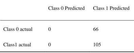
Result is shown in form of confusion matrix. Confusion matrix, tells about total number of true positive and true negative values.[6] As this is the two class problem so matrix will be the order of 2*2.

Class 0 Predicted Class 1 Predicted

Class 0 actual 0 66

Class1 actual 0 105

Fig 6: Confusion matrix

1*1 shows true-positive, 1*2 shows false-positive, 2*1 shows false-negative, 2*2 shows false-negative.

The problem using SVM classifier is, it is predicting right false-negative values but for true-positive it is not predicting any value. It signifies that every value belongs to only one class.

Results according to classification report:

Fig. 7: Confusion matrix report

Precision: It shows that out of examples that the learning algorithm marked as positive, how many are correctly positive which in this model is depicted as 38% which is quite low. Mathematical formulae: Tp/ (Tp + Fp)

Tp - true positive (training example which are true and classifier also predicted them true.)

Fp - false positive (training example which are false but classifier predicted them true.)

Recall: To study how many of positive example in the learning algorithm is retrieved as positive.

Mathematical formulae: Tp/ (Tp + Fn) Fn = False negative.

This is also called true positive rate.

F1-score: it is generally required to find balance between precision and recall, for the problem the main focus is to get better result for precision and recall only as it will automatically enhance the f1-score.

Model 2: Enhancing the results with grid search: [6] Before fitting the data to SVM model it is better to find out the best arguments for c and gamma parameters; which is best suited for the given problem and this can be done by using grid search. Grid search is a process that allows using the right parameters by trying all the best possible parameters. [3]. It is like a hit and trail method in which certain values have to be passed in dictionary called GridSearchCV. Instead of using default values for SVM parameters, model will try the arguments given in the GridSearchCV dictionary and compare the final result with all passed arguments. Lastly, gives the best set of arguments to use.

GridSearchCV uses a dictionary that describes the parameters that should be tried in a model to train. In this dictionary, keys are the parameters and values are the list of settings that need to be tested.

Fig. 9: Creating parameters lists

So these are the gamma and c values to be tried for this classifier.

Fig. 10: Initializing grid search

The higher the verbose value the more description it is going to give about the grid search process in result.

Fig. 11: Grid search results

Firstly it will run with the same loop with cross validation to find best parameter combinations. Once it has the best combination it will fit again to build a single new model using the best parameters settings. Best parameter settings can be seen by:

Fig.12: Best parameters

As these are the best parameters so now these C and gamma values should be used for creating the classifier.

Prediction with C = 10 and gamma = 0.0001

Fig. 13: Fitting data using grid search values

Fig. 14: Confusion matrix after grid search

Class 0 Predicted Class 1 Predicted

Class 0 Actual 60 6

Class 1 Actual 3 102

Now classifier is predicting values from both the classes unlike the previous results.

Fig. 15: Classification matrix report after grid search

For both the classes precision and recall are above 90 percent, which is a really good result.

3.

RESULTS

3.1

Comparison of result of both models

with or without grid search in terms of

precision-recall curve:

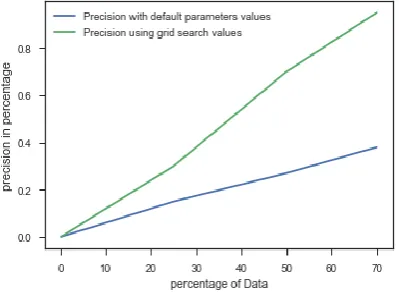
The following graph represents the comparison between precision (before and after using grid search). X axis - percentage of data used, as for training data used is 70 percent of total given data.

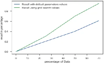
The following graph represents the comparison between recall (before and after using grid search)

Fig. 17: Line graph comparing recall

3.2

Tables illustrating average recall and

average precision

Table 2: SVM with and without Grid search

SVM Model Avg.Recall Avg. Precision

without grid

search 38% 61%

with grid search 95% 95%

3.3

Increase in performance of model

Fig. 18: Bar graph of avg. results

3.3.1

Classification Report:

The blue area of every bar represents the average score of precision, recall, and F1-score before the grid search. The pink area of every bar displays the increase in score after applying grid search.

Table 3: (all numerical data in percentage)

SVM Model

Avg.

Precision Avg. Recall

Avg. F1-score

Height of

blue bar 38 61 47

Height of

pink bar 95 95 95

Result enhanced

by

57 34 48

From the results shown in table 3 and Fig.18 it is clear that with help of grid search average precision is increased by 57 percent, average recall is increased by 34 percent and average F1-score is increased by 48 percent.

4.

CONCLUSION

This paper has shown the comparative results using SVM functions with and without grid search. It is clear with the obtained results depicted in Fig 16, 17 and 18, that using grid search with Breast cancer dataset gives much better result than using normal SVM model. The experiment results are encouraging. It can be seen that right value of parameters for C and gamma is critical for a given amount of data. This model can be used in establishing the predictions for other diseases also which can work as a decision support system in health care sector.

5.

REFERENCES

[1] Bemmel J.H.V. (1984). The structure of medical informatics. Med Inform. 9(3-4). Pp. 175–180.

[2] Shortliffe, E.H., Blois, M.S. (2006). The computer meets medicine and biology: the emergence of a discipline. In: Shortliffe EH, editor. Biomedical informatics: computer applications in health care and biomedicine. Springer Science+ Business Media, LLC; New York, NY: pp. 3– 45.

[3] Bray F, Ferlay J, Soerjomataram I, Siegel RL, Torre LA, Jemal A. Global Cancer Statistics 2018: GLOBOCAN estimates of incidence and mortality worldwide for 36 cancers in 185 countries. CA Cancer J Clin, in press

Retrieved from:

https://www.wcrf.org/dietandcancer/cancer-trends/breast-cancer-statistics

[4] Breast Cancer Research Foundation (n.a), Breast Cancer Statistics, Retrieved From: https://www.bcrf.org/breast-cancer-statistics

[5] Pierce, B.G. and Wallace, C. (1971). University of Colorado Medical Center, Denver, Cancer Research.

Retrieved From:

http://cancerres.aacrjournals.org/content/canres/31/2/127. full.pdf

[6] Wolberg, H.W., Street, N.W., & Mangasarian, L.O., (n.a). Breast Cancer Wisconsin (Diagnostic) Data Set. UCI Machine learning Repository. Retrieved From: [7] Theodoros, E., & Pontil, M. (2001). Support Vector

Machines: Theory and Applications. 2049. 249-257. 10.1007/3-540-44673-7_12. Retrieved From: https://www.researchgate.net/publication/221621494_Su pport_Vector_Machines_Theory_and_Applications. [8] Visa, S & Ramsay, B. & Ralescu, A. & Knaap, E.

(2011). Confusion Matrix-based Feature Selection. CEUR Workshop Proceedings. 710. 120-127.

[9] Retrieved From:

https://www.researchgate.net/publication/220833270_Co nfusion_Matrix-based_Feature_Selection