A Poisson Solver Based on Iterations on a Sylvester System

ISSN Online: 2152-7393 ISSN Print: 2152-7385

DOI: 10.4236/am.2018.96052 Jun. 29, 2018 749 Applied Mathematics

A Poisson Solver Based on Iterations on a

Sylvester System

Michael B. Franklin, Ali Nadim

Institute of Mathematical Sciences, Claremont Graduate University, Claremont, CA, USA

Abstract

We present an iterative scheme for solving Poisson’s equation in 2D. Using fi-nite differences, we discretize the equation into a Sylvester system,

AU UB F+ = _{, involving tridiagonal matrices A and B. The iterations occur}

on this Sylvester system directly after introducing a deflation-type parameter that enables optimized convergence. Analytical bounds are obtained on the spectral radii of the iteration matrices. Our method is comparable to Succes-sive Over-Relaxation (SOR) and amenable to compact programming via vec-tor/array operations. It can also be implemented within a multigrid frame-work with considerable improvement in performance as shown herein.

Keywords

Poisson’s Equation, Sylvester System, Multigrid

1. Introduction

Poisson’s equation _{∇ =}2_{u f , an elliptic partial differential equation [1], was first} published in 1813 in the Bulletin de la Société Philomatique by Siméon-Denis Poisson. The equation has since found wide utility in applications such as elec-trostatics [2], fluid dynamics [3], theoretical physics [4], and engineering [5]. Due to its expansive applicability in the natural sciences, analytic and efficient approximate solution methods have been sought for nearly two centuries. Ana-lytic solutions to Poisson’s equation are unlikely in most scientific applications because the forcing or boundary conditions on the system cannot be explicitly represented by means of elementary functions. For this reason, numerical ap-proximations have been developed, dating back to the Jacobi method in 1845. The linear systems arising from these numerical approximations are solved ei-ther directly, using methods like Gaussian elimination, or iteratively. To this

How to cite this paper: Franklin, M.B. and Nadim, A. (2018) A Poisson Solver Based on Iterations on a Sylvester System. Ap-plied Mathematics, 9, 749-763.

https://doi.org/10.4236/am.2018.96052

Received: June 1, 2018 Accepted: June 26, 2018 Published: June 29, 2018

Copyright © 2018 by authors and Scientific Research Publishing Inc. This work is licensed under the Creative Commons Attribution International License (CC BY 4.0).

http://creativecommons.org/licenses/by/4.0/

DOI: 10.4236/am.2018.96052 750 Applied Mathematics day, there are applications solved by direct solvers and others solved by iterative solvers, depending largely on the structure and size of the matrices involved in the computation. The 1950s and 1960s saw an enormous interest in relaxation type methods, prompted by the studies on optimal relaxation and work by Young, Varga, Southwell, Frankel and others. The books by Varga [6] and Young [7] give a comprehensive guide to iterative methods used in the 1960s and 1970s, and have remained the handbooks used by academics and practi-tioners alike [8].

The Problem Description

The Poisson equation on a rectangular domain is given by

{

}

2_{u f in x y, | 0 x a,0 y b}

∇ = Ω = ≤ ≤ ≤ ≤ (1)

where u u x y=

(

,

)

_{is to be solved in the 2D domain} Ω_{, and} f x y

( )

, is the forcing function. Typical boundary conditions for this equation are either Di-richlet, where the value of f x y

( )

, is specified on the boundary, or Neumann, where the value of the normal derivative is specified on the boundary. These are given mathematically as,

ˆ

or on ,

D N

u g= ∂ ∂ ≡ ⋅∇ =u n n u g ∂Ω (2) where nˆ is the outward unit normal along ∂Ω _and g_D and gN are the

function values specified by Dirichlet or Neumann boundary conditions. It is also possible to have mixed boundary conditions along the boundary, where some edges have Dirichlet and some have Neumann, so long as the problem is well-posed. Furthermore, edges could be subject to Robin boundary conditions of the form c u c u n g1 + ∂ ∂ =2 R. Any numerical scheme designed to solve the

Poisson equation should be robust in its ability to incorporate any form of boundary condition into the solver. A detailed discussion of boundary condition implementation is given in the Appendix. Discretizing (1) using central differ-ences with equal grid size ∆ = ∆ =x y h leads to an M N× rectangular array of unknown U, such that Ui j, ≈u x y

(

i, j

)

(assuming that a and b are both integer

multiples of h). This discretization leads to a linear system of the form AU UB F+ = _{, the Sylvester equation, which can be solved either directly or}

ite-ratively. The direct method utilizes the Kronecker product approach [9], given by

(

)

(

T

)

where kron , kron ,

Ku f= K= I A + B I (3)

where u and f are appropriately ordered MN×1 _{column vectors obtained} from the M N× _{arrays U and F, and K is a sparse} MN MN× _{matrix. The}

Kronecker product, kron ,

(

P Q

)

, of any two matrices P and Q is a partitioned matrix whose ijth _{partition contains matrix Q multiplied by component}

ij

p of

DOI: 10.4236/am.2018.96052 751 Applied Mathematics

int int int_,

AU +U B F= ₍₄₎

where _Uint _{is the m n× array of interior unknowns (not including the known} boundary values when Dirichlet boundary conditions are given) with

2

m M= − _and n N= −2_{. Operator matrices A and B are given by the O h}

( )

2 finite difference approximation to the second derivative,

2

2 1 1 2 1

1 _.

1 2 1 1 2 h

−

 

 ₋ 

 

 

 ₋ 

 

 ₋ 

 

   (5)

For an array of unknowns _Uint_∈m n× _{, the operator matrices are of} dimen-sion _A∈m m× _{, and B∈}n n× _{. The matrix structure of U should be modified} such that the first index i corresponds to the x-direction, and the second index j

corresponds to the y-direction. With this orientation, multiplying _Uint _{by the} matrix A on the left approximates the second derivative in the x-direction, and multiplying _Uint _{by the matrix B on the right approximates the second} deriva-tive in the y-direction.

2. Sylvester Iterative Scheme

Examining (4) it might seem natural to move one term to the right-hand side of the equation to achieve an iterative scheme such as:

AU UB F+ = ⇒ AU F UB= −

1 1 1 _,

k k

U + A F A U B− −

⇒ = − ₍₆₎

However, this scheme diverges, and an alternative approach is required to ite-rate on the Sylvester system. An appropriate method is to break up the iterative scheme into two “half-steps’’ as follows

1) First half-step: _Uk _→U*

(

)

AU F UB= − ⇒ A−αI+αI U F UB= −

(

_A

_α

_{I U}

)

* _{F U B}k

(

_α

_I

)

⇒ − = − + (7)

2) Second half-step: _U*_→Uk+1

(

)

UB F AU= − ⇒ U B−βI+βI = −F AU

(

)

(

)

1 *

k

U + B

β

I F A

β

I U

⇒ − = − + ₍₈₎

where _U* _{is some intermediate solution between steps k and k+1.} Rearrang-ing, this leads to

*

1 *

1 1 _{1 ,}

1 1 _{1 .}

k

k

I A U U I B F

U I B I A U F

α α α

β β β

+

 ₋  ₌  ₊ ₋

   

   

   

− = + −

   

   

(9)

DOI: 10.4236/am.2018.96052 752 Applied Mathematics formulation [10], where Poisson’s equation is reformulated to have pseudo-time dependency,

d _,

dU AU UB Ft = + − (10) which achieves the solution to Equation (4) when it reaches steady-state. This method is separated into two half-steps, the first time step going from time

1 2

k→ +k treating the x-direction implicitly and the y-direction explicitly. The second time step then goes from time k+1 2→ +k 1_{, treating the}

y-direction implicitly and the x-direction explicitly. The two half-steps are, 1 2

1 2 2

1 1 2

1 2 1

2 1 _, 2 1 _, 2 k k k k k k k k

U U _{AU U B}

t h

U U _{AU U B}

t h + + + + + + − _{ } = _ + _ ∆ − _{=  + }   ∆ (11)

which leads to

1 2

1 1 2

,

2 2 2

.

2 2 2

k k

k k

t t t

I A U U I B F

t t t

U I B I A U F

+ + + ∆ ∆ ∆  ₋  ₌  ₊ ₋         ∆ ∆ ∆  ₋  _{= +}  ₋         (12)

This iteration procedure looks nearly identical to our Sylvester iterations giv-en in (9) with ∆t 2 replaced by the unknown parameters 1/α and 1/β. However in our formulation, there is no pseudo-time dependency introduced. Instead, the eigenvalues of our operator matrices A and B are deflated to produce an iterative scheme that optimally converges, and finding the values of the parameters α and

β becomes an optimization problem.

Convergence

After the Sylvester Equation (4) is modified into the iterative system (9), the iterative scheme can be written as a single step by substituting the expression for the intermediate solution _U* _{into the second step of the iterative process; this} yields the single update equation for _Uk+1 _{given by}

1 1

1

1 1

1 1 1 1

1 1 1 1 1 _.

k k

U I A I A U I B I B

I A I A I F I B

β α α β

α β α β β

− − + − −       =_ + _ − _{ } + _ − _          _{  }  _{ } −  + _ − _ −   −          (13)

Assuming that an exact solution _Uexact _{exists that exactly satisfies the linear} system (4), i.e. _AUexact_+Uexact_{B F= , we define the error between the k}th

itera-tion and the exact soluitera-tion as

exact_.

k k

in-DOI: 10.4236/am.2018.96052 753 Applied Mathematics volving the forcing F disappear, we arrive at

1 _,

k k

E + ₌PE Q ₍₁₅₎

where the matrices P and Q are given by

1 1

1 1 _, 1 1 _.

P I A I A Q I B I B

β α α β

− −

     

=_ + _ − _ =_ + _ − _

   

    (16)

Denoting the m eigenvalues of _A∈m m× _by A k

λ , and the n eigenvalues of

n n

B_∈× _by B k

λ _{, the corresponding deflated eigenvalues of the iteration}

ma-trices P and Q are

(

)

(

)

(

)

(

)

1

, 1,2, , , 1

1

, 1,2, , . 1

A _A

k

P k

k A A

k k

B _B

k

Q k

k B B

k k

k m

k n

λ β _{α β λ}

λ

β α λ λ α

λ α _{β α λ}

λ

α β λ λ β +  +  = = _{ } = − − _{ } + _{ + } = =   = − − _{ }   (17)

A sufficient condition for convergence of the iterative process is achieved if the spectral radii of both iteration matrices P and Q are less than one,

( )

max P 1 and

( )

max Q 1.

k k

P Q

ρ ≡ λ < ρ ≡ λ < (18)

The error at each consecutive iteration is decreased by the product of ρ

( )

P

and ρ

( )

Q _,

( ) ( )

( ) ( )

(

)

1 1 1 0 , , , k k k k k k

E PE Q

E P Q E

E P Q E

ρ ρ ρ ρ + + + = = = (19)

where _E0 _{is the initial error. Often in practical applications, the exact solution} is not known, so the error _Ek _{cannot be computed directly. In this case, the}

preferred measure in iterative schemes is given by the residual, which measures the difference of the left and right hand sides of the linear system being solved. This will be further discussed in the Results section.

3. Finding Optimal Parameters

α

and

β

Finding α and β is an optimization problem for achieving the fastest conver-gence rate of the Sylvester iterative scheme (9). Given the operator matrices A

and B and their respective eigenvalues A k

λ and B k

λ , it seems feasible to find optimal values of α and β to minimize the spectral radii of the iteration matrices

P and Q given in Equations (17). From (15) the error _Ek+1 _{is found by} multip-lying by P on the left, and Q on the right, thus the convergence is governed by the spectral radii of both P and Q.

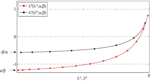
Figure 1 shows the eigenvalues of P and Q for arbitrary m and n, given by Equation (17), plotted vs. the eigenvalues of A and B for some parameters α and

β. It can be seen that as _λA _{or λ}B _{get large in magnitude, the values of λ}P

[image:6.595.213.532.75.247.2]

DOI: 10.4236/am.2018.96052 754 Applied Mathematics

Figure 1. Eigenvalues _{λ λ α β}P

(

A; ,

)

_{and λ λ α β}Q

(

B_{; ,}

)

_{vs. λ}Q _{and λ}B _{for given} constant α _and β_{. In this figure,} α β> , so ρ

( )

P =α β> 1, and the scheme will diverge.

the high frequency eigenvalues of P and Q, in magnitude, will be greater than one, thus convergence condition (18) will not be satisfied. This provides the re-striction for convergence that,

.

α β= ₍₂₀₎

This optimal value of α β= _{will henceforth be called α}*_{. It is important to} note that the operator _A∈m m× _{or B∈}n n× _{with the larger dimension}

(

)

max , ,m n

≡

 (21) has a larger range of eigenvalues. Figure 1 shows m n> , (i.e. _=m_{) so it can} be seen that min

( )

_λA _<min

( )

_λB _{and max}

( )

_λA _>max

( )

_λB _{. This property of}

the eigenvalues is important when calculating an expression for _c, which will soon prove to be a highly useful parameter for an adaptive approach to smooth-ing. Letting _{α β α= =} * _{in (17) gives the following expression for the} eigenva-lues of P and Q:

*

*

*

*

, 1,2, , ,

, 1,2, , .

A

P k

k A

k B

Q k

k B

k

k m

k n

α λ

λ

α λ

α λ

λ

α λ

+

= =

− +

= =

−





(22)

Finding the optimal parameter _α* _{is done by considering the error} reduc-tion of Sylvester iterareduc-tions on an arbitrary initial condireduc-tion U0. Assume that U0

can be decomposed into its constituent error (Fourier) modes, ranging from low frequency (smooth) to high frequency (oscillatory) modes. Given that U0

con-tains error modes of all frequencies, the most conservative method would be to choose _α* _{such that the spectral radii ρ}

( )

_{P and ρ}

( )

_{Q are minimized over} the full range of frequencies. This ensures that all modes of error are efficiently relaxed, and convergence is governed by the product of spectral radii.

[image:7.595.213.534.72.240.2]

DOI: 10.4236/am.2018.96052 755 Applied Mathematics

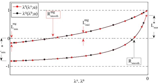
Figure 2. Eigenvalues _{λ λ α}P

(

A;

)

_{and λ λ α}Q

(

B_;

)

_{illustrating the quantities involved in} computing the optimal parameters _α* _and *

mg

α , and their respective optimal smoothing regions *

smooth

R and mg smooth

R . Note that the upper curve illustrates the method of determining _α* _{in the multigrid formulation, while the lower curve is for} determining _α* _{in conservative Sylvester iterations.}

determining _α* _{would be to set} * * min max

L =L _{and according to (22),}

* *

max min

* *

min max

.

A A

A A

α λ

α λ

α λ α λ

 

 +  +

− ₋ =  ₋ 

    (23)

Noting that eigenvalues for all dimensions collapse onto the curves shown in Figure 2, this conservative approach “locks in’’ the value of the larger operator’s spectral radius, thus providing an upper bound for convergence. Figure 2 shows m n> , so ρ

( )

P >ρ

( )

Q , so convergence will be limited by ρ

( )

P . Equation (23) can then be solved for _α* _giving

(

)

(

)

*

min min max max

min A , B max A , B ,

α = λ λ × λ λ ₍₂₄₎

where absolute values are introduced as a reminder that

_{λ λ}

A, B _{are negative.}

This value of the parameter _α* _{most uniformly smooths all frequencies for any} arbitrary U0 containing all frequency modes of error. It can be seen that the spectral radii of P and Q shown in Figure 2 occur at either endpoint, and the minimum amplitude occurs near the intersection of the curve with the axis. Va-rying the parameter _α* _{in (22) controls the intersection point, and thus creates} an effective “optimal smoothing region’’, denoted Rsmooth∗ . Modes of error asso-ciated with this optimal smoothing region will be damped fastest, which makes Sylvester iterations highly adaptive in nature. This adaptive nature of Sylvester iterations lends itself nicely to a multigrid formulation.

DOI: 10.4236/am.2018.96052 756 Applied Mathematics shown in the upper curve of Figure 2. The height mg

mid

L is essentially the dis-tance above the axis associated with the approximate “middle’’ eigenvalue in the range of _λA _{or λ}B_{. This equality gives the following optimal parameter value}

for the Sylvester multigrid method

(

)

(

)

mg min minA , minB min midA , midB ,

α∗ ₌ λ λ _× λ λ ₍₂₅₎

where, if m n≠ , the minimum (i.e., most negative) middle eigenvalue

(

)

mid min max 2

λ ≡ λ +λ _{is chosen to shrink the optimal smoothing region} mg smooth

R

such that high frequencies are smoothed most effectively. This choice of optimal parameter can be observed in Figure 2 to drastically decrease the magnitude of

P

λ and _λQ _{associated with high frequencies which significantly enhance}

re-laxation in accordance with the multigrid philosophy. To find analytical expressions for _α* _and

mg

α

∗ _{, it is necessary to have values} for _λA _{and λ}B_{. For Dirichlet boundary conditions, analytical expressions for}

A

λ _{and λ}B _{are derived below, but for Neumann boundary conditions}

numer-ical approaches are necessary to find _λA _{and λ}B_{. The operator matrices A and} B are each of tridiagonal form,

0 1

1 0 1

1 0 1

1 0

.

p p

d d

d d d

d d d

d d

×

 

 

 

  ∈

 

 

 

 

    (26)

Tridiagonal matrices with constant diagonals, such as A and B for Dirichlet boundary conditions, have analytical expressions for their eigenvalues given by

0 2 cos1 π₁ , 1,2, ,

k d d _pk k p

λ = + _ _ =

+

   (27)

where p is the arbitrary dimension of the matrix [12]. Neumann boundary condi-tions alter the upper and lower diagonals of A or B, thus there is no analytical form of eigenvalues for Neumann boundary conditions. Using (5) and (27) gives the following analytic form of the eigenvalues of the tridiagonal matrices A and B,

2

2 _{1 cos} π _{, 1,2, , ,}

1

k _{h p}k k p

λ = − +  ₊  =

 

   (28)

which achieves minimum and maximum values given by

min 2 max 2

2 _{1 cos} π _and 2 _{1 cos} π _,

1 1

p

p p

h h

λ = − +  ₊  λ = − +  ₊ 

   

    (29)

respectively. Using (24), (25), and (29) the analytic expressions for optimal pa-rameters for both conservative and multigrid approaches are given by

* 2

mg 2

2 _{1 cos} π _{1 cos} π _,

1 1

2 _{1 cos} π _{2 cos} π _cos π _,

1 1 1

h

h α

α∗

    

= _− + _{ }− + _{ }

+ +

   

  

      

= _− + _{ }− + _{ }+ _{ }

+ + +

     

  



 

 

  

DOI: 10.4236/am.2018.96052 757 Applied Mathematics where again ≡max ,

(

m n

)

. Having expressions for _α* _and

mg

α∗ _{allows λ}P

and _λQ _{to be found analytically using (22) which subsequently allows the}

spectral radii of the iteration matrices P and Q to be calculated. Knowing the spectral radii of the iteration matrices P and Q is highly advantageous, as it al-lows for an analysis of the Sylvester iterative scheme.

4. Analysis

The analysis of standard Sylvester iterations can be performed and describes the error reduction with each consecutive iteration using (19). Having the optimal parameters given by (30) and eigenvalues of P and Q in (22), the spectral radii can be calculated to be

( )

( )

π π π

1 cos 1 cos 1 cos

1 1 1

,

π π π

1 cos 1 cos 1 cos

1 1 1

π π π

1 cos 1 cos 1 cos

1 1 1

1 c m m P m m n n Q ρ ρ          − + _{ }+ _− + _{ }− + _{ } + + +        =          − + _{ }− _− + _{ }− + _{ } + + +                 − + _{ }+ _− + _{ }− + _{ } + + +        = − +          .

π π π

os 1 cos 1 cos

1 1 1

n n     _{− − +}   _{− +}    ₊    ₊   ₊            (31)

Rewriting the last expression of (19), we see that

( ) ( )

(

)

0 ~ .

k

k

E

P Q

E ρ ρ (32)

If we want to reduce our error to _Ek _{~ E}0 _{and we wish to know how} many iterations it will take to achieve this error reduction, using (32) we set

( ) ( )

(

ρ

P

ρ

Q

)

k~, and solving for k, we find it will take

( )

( ) ( )

(

log

)

~ log k P Q ρ ρ  (33)

iterations to reduce the error by . Here log can be with respect to any base, as long as the same one is used in both the numerator and denominator; e.g., the natural log can be used. Recall that the exact solution _Uexact _{of (4) is only an}

approximate solution of the differential Equation (1) we are actually solving. Due to this, we can only expect accuracy of the truncation error of the approxi-mation. With an _{O h}

( )

2 _method, exact

,

i j

U differs from U x y

(

i, j

)

on the order

of _h2 _{so we cannot achieve better accuracy than this no matter how well we} solve the linear system. Thus, it is practical to take  to be something propor-tional to the expected global error, e.g. _=Ch2 _{for some fixed C[12].}

To calculate the order of work required asymptotically as h→0_{, (i.e.} m→ ∞_{) using (33) and our choice for} , we see that

DOI: 10.4236/am.2018.96052 758 Applied Mathematics The expressions for ρ

( )

P _and ρ

( )

Q _{in (31) contain several cosine terms}

which can be Taylor expanded about different values. Cosines with arguments like πx can be expanded about x=1 _or x=0 _{depending on the form of x,} namely

( )

(

)

(

(

)

)

( )

( )

2

2 3

2

2 3

π

cos π ~ 1 1 1 for 1, 2

π

cos π ~ 1 for 0, 2

x x x x

x x x x

− + − + − ≈

− + ≈





(35)

where, from (31), the form of x is something like m m

(

+1

)

_or 1

(

m+1

)

_,

which clearly approach one or zero, respectively, in the limit that m→ ∞. Using these expansions, along with the fact that _{1 1}

(

_−x

)

_{~ 1+ +x O x}

( )

2 _{for x1 to} simplify the spectral radii, we arrive at the following

( )

~

( )

~ 1 π 1 π 2,

1 4 1

P Q

ρ ρ − _{+ } _

+  + 

  (36)

when m n, 1. Since h=1

(

m+1

)

_{, (34) combined with (36) gives the}

follow-ing order of work needed for convergence to within _~Ch2_:

(

)

_{( )}

2log 1

~ ~ log ,

π

2log 1 1

m

k − +_π m

 ₋ 

 ₊ 

 





(37)

where only linear terms are used from (36), and the latter simplified expression can be deduced by using the property that _{log 1}

(

_+x

)

_{~x O x+}

( )

2 _{for x1.} Note that when m n= _{, the order of work for Sylvester iterations is}

(

) ( )

~ π log

k m m , which is comparable to the work necessary for the Successive Over-Relaxation (SOR) algorithm to solve Poisson’s equation [12]. This will be our basis for comparison in the Results section for standard Sylvester iterations.

5. Results

Problems solved by Sylvester iterations can, in general, be written shorthand as U F=

 , where  is a linear operator. In the case of Poisson’s equation,  is the Laplacian operator. As an error measure, the discrete ⋅ _{2 norm of the}

residual, r F≡ −_U_{, can be measured at each iteration. This number provides} the stopping criterion for our iterative schemes, namely the iterations are run until

( )k ( )k _tol ( )0 _,

r = F−U < × r (38)

where _r( )0 _{is the initial residual, and tol is the tolerance. The tolerance is set to} machine precision _{tol ~ 10}−16 _{to illustrate the asymptotic convergence rate,}

( ) ( ) ( )1 ,

k k

k

r q

r −

= (39)

DOI: 10.4236/am.2018.96052 759 Applied Mathematics Mac PowerPC G4. The model problem that is solved is given by

(

)(

) (

)(

)

2 ₂ 2 _{1 6} 2 ₁ 2 2 _{1 6} 2 ₁ 2 _{in ,}

0 on ,

u y x y x y x

u

 

∇ = − _ − − + − − _ Ω

= ∂Ω (40)

where Ω =

{

x y, | 0≤ ≤x 1,0≤ ≤y 1

}

_{, and whose exact solution}

(

)

(

)(

)

exact _, 2 4 4 2 _,

u x y = x −x y −y (41)

is known so errors can be computed [11]. This model problem is used to show performance of both standard and multigrid Sylvester iterations. In all cases, the initial guess _U( )0 _{of the iterative scheme is a normalized random array and can} be assumed to contain all modes of error.

5.1. Standard Sylvester Iterations

For comparison, standard Sylvester iterations were tested against Successive Over-Relaxation (SOR) with Chebyshev acceleration (see e.g., [13]). In SOR with Chebyshev acceleration, one uses odd-even ordering of the grid and changes the relaxation parameter

ω

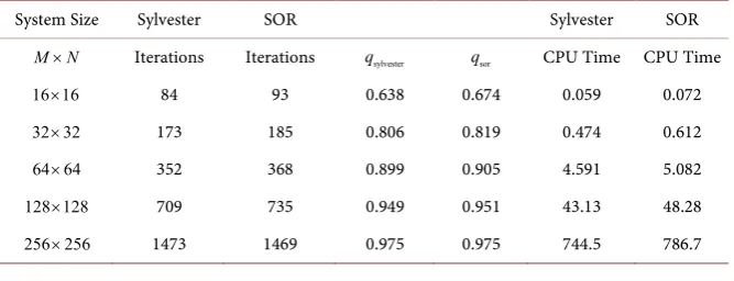
at each half-step, which converges to the optimal re-laxation parameter. The results are shown in Table 1. It is important to note that SOR iterations involve no matrix inversions, whereas Sylvester iterations do, thus the CPU time measure might not be an appropriate gauge for this particular comparison. From these results, it is clear that standard Sylvester iterations are comparable to SOR, and in most cases, converge to within tolerance in fewer iterations than SOR. An unfortunate artifact of standard iterative schemes is that as system size increases, so does the spectral radii governing the convergence. This can be observed in Table 1, as asymptotic convergence rates for each me-thod qsylvester and qsor steadily increase, thus requiring higher numbers of ite-rations to solve within tolerance. The number of Sylvester iteite-rations required to converge is consistent with the predicted number of iterations given by Equation (33) letting _{=tol 10=} −16_.

5.2. Multigrid Sylvester Iterations

[image:11.595.207.541.595.723.2]

In multigrid Sylvester iterations, the performance of the V

(

ν ν1, 2

)

-cycle using Sylvester iterations is compared to that using the traditional Gauss-Seidel (GS)

Table 1. Sylvester iterations vs. successive over-relaxation (SOR).

System Size Sylvester SOR Sylvester SOR

M N× Iterations Iterations qsylvester qsor CPU Time CPU Time

16 16× _{84 93 0.638 0.674 0.059 0.072}

32 32× 173 185 0.806 0.819 0.474 0.612

64 64× _{352 368 0.899 0.905 4.591 5.082}

128 128× 709 735 0.949 0.951 43.13 48.28

[image:12.595.207.540.89.227.2]

DOI: 10.4236/am.2018.96052 760 Applied Mathematics

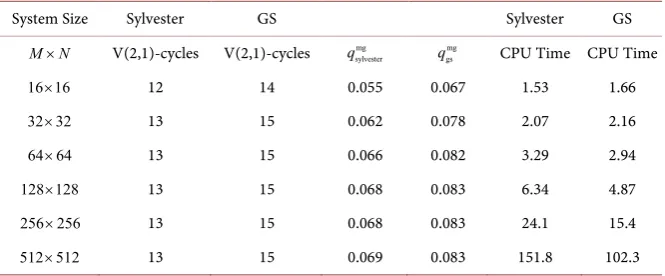
Table 2. Multigrid sylvester iterations vs. multigrid gauss-seidel (GS) iterations.

System Size Sylvester GS Sylvester GS

M N× _{V(2,1)-cycles V(2,1)-cycles} mg sylvester

q mg

gs

q CPU Time CPU Time 16 16× _{12 14 0.055 0.067 1.53 1.66}

32 32× _{13 15 0.062 0.078 2.07 2.16}

64 64× 13 15 0.066 0.082 3.29 2.94

128 128× _{13 15 0.068 0.083 6.34 4.87}

256 256× 13 15 0.068 0.083 24.1 15.4

512 512× _{13 15 0.069 0.083 151.8 102.3}

iterations. The parameter ν1 represents the number of smoothing iterations done on each level of the downward branch of the V-cycle, while ν2 represents the number done on the upward branch. In practice, common choices are

1 2 3

ν ν ν= + ≤ _{, so our performance is based on the} V

( )

2,1 -cycle [14]. In each case, the V-cycle descends to the coarsest grid having gridwidth h0=1 2, and in the Sylvester implementation, the value of

α

mg∗ is calculated to smooth high frequencies most effectively on each grid traversed by the cycle. The results are shown in Table 2. It can be seen that the asymptotic convergence rates mg

sylvester q and mg

gs

q reach steady values independent of the gridwidth h. This is characte-ristic of multigrid methods, and enables the optimality of the multigrid method. It is clear when comparing the CPU times of the Sylvester multigrid formulation in Table 2 with standard Sylvester iterations in Table 1 that the multigrid framework is substantially faster (e.g., 30 times faster than standard iterations for a grid of size 256 256× _{). It can also be seen that the asymptotic convergence}

rates are such that mg mg sylvester gs

q <q _{, thus convergence is met in fewer} V

_{( )}

2,1

cycles using Sylvester smoothing versus Gauss-Seidel smoothing.

6. Conclusion

Sylvester iterations provide an alternative iterative scheme to solve Poisson’s eq-uation that is comparable to SOR in the number of iterations necessary to con-verge, namely converging to discretization accuracy within k~

(

m π

) ( )

log m

iterations. The true benefit of the Sylvester iterations, however, comes from its adaptive ability to smooth any range of error frequencies, thus being a perfect candidate for smoothing in a multigrid framework. Multigrid V

( )

2,1 -cycles using Sylvester smoothing have an asymptotic convergence rate of

mg

sylvester 0.069

q = _(versus mg

gs 0.083

q = _{for Gauss-Seidel smoothing) and indicate}

significant improvement in efficiency over standard Sylvester iterations.

References

DOI: 10.4236/am.2018.96052 761 Applied Mathematics [2] Feig, M., Onufriev, A., Lee, M.S., Im, W., Case, D.A. and Brooks III, C.L. (2003) Performance Comparison of Generalized Born and Poisson Methods in the Calcu-lation of Electrostatic Solvation Energies for Protein Structures. Journal of Compu-tational Chemistry, 25, 265-284. https://doi.org/10.1002/jcc.10378

[3] Ravoux, J.F., Nadim, A. and Haj-Hariri, H. (2003) An Embedding Method for Bluff Body Flows: Interactions of Two Side-by-Side Cylinder Wakes. Theoretical and Computational Fluid Dynamics, 16, 433-466.

https://doi.org/10.1007/s00162-003-0090-4

[4] Trellakis, A., Galick, A.T., Pacelli, A. and Ravaioli, U. (1997) Iteration Scheme for the Solution of the Two-Dimensional Schrodinger-Poisson Equations in Quantum Structures. Journal of Applied Physics, 81, 7880-7884.

https://doi.org/10.1063/1.365396

[5] Saraniti, M., Rein, A., Zandler, G., Vogl, P. and Lugli, P. (1996) An Efficient Multi-grid Poisson Solver for Device Simulations. IEEE Transactions on Computer-Aided Design of Integrated Circuits and Systems, 15, 141-150.

https://doi.org/10.1109/43.486661

[6] Varga, R.S. (1962) Matrix Iterative Analysis. Prentice-Hall, New Jersey.

[7] Young, D.M. (1971) Iterative Solution of Large Linear Systems. Academic Press, New York.

[8] Brezinski, C. and Wuytack, L. (2001) Numerical Analysis: Historical Developments in the 20th Century. Elsevier Science B.V., Netherlands.

[9] Van Loan, C.F. (2000) The Ubiquitous Kronecker Product. Journal of Computa-tional and Applied Mathematics, 123, 85-100.

https://doi.org/10.1016/S0377-0427(00)00393-9

[10] Peaceman, D.W. and Rachford, H.H. (1955) The Numerical Solution of Parabolic and Elliptic Differential Equations. Journal of the Society for Industrial and Applied Mathematics, 3, 28-41. https://doi.org/10.1137/0103003

[11] Briggs, W.L., Henson, V.E. and McCormick, S.F. (2000) A Multigrid Tutorial. 2nd Edition, Society for Industrial and Applied Math, Philadelphia.

https://doi.org/10.1137/1.9780898719505

[12] LeVeque, R.J. (2007) Finite Difference Methods for Ordinary and Partial Differen-tial Equations: Steady-State and Time-Dependent Problems. Society for Industrial and Applied Math, Philadelphia. https://doi.org/10.1137/1.9780898717839

[13] Press, W., Vetterling, W., Teukolsky, S. and Flannery, B. (1992) Numerical Recipes in Fortran. 2nd Edition, Cambridge University Press, New York.

DOI: 10.4236/am.2018.96052 762 Applied Mathematics

Appendix

1) Boundary condition implementation

Solving the Poisson equation using Sylvester iterations lends itself nicely to boundary condition implementation. Dirichlet boundary conditions of the form

( )

0, 1

( )

,

(

,

)

2

( )

,

( )

,0 3

( )

,

( )

, 4

( )

,

u y =u y u a y =u y u x =u x u x b =u x ₍₁₎

where u u u1, ,2 3 and u4 are functions describing the edges of U, can be im-plemented as follows. The unknown values in the Sylvester system given in Equ-ation (4) are the m n× array of interior values, where m M= −2,n N= −2_{. It} is possible to incorporate Dirichlet boundary conditions directly into this inte-rior system by examining the partitioned matrix product, for example AU, given by

(2)

with UB taking an analogous partitioned form. Multiplying through by _h2 as-sociated with the operator matrices A and B, the partitioned Sylvester system for internal unknowns gives

( )( )

( )( )

( )( )

T int int T T int int T 2 int

1 2 3 4 ,

L R T B

A ⋅u + A U +A ⋅u +u ⋅B + U B +u ⋅B = h F (3)

where all matrix-vector products are m n× _{outer products. Note that the}

product AU incorporates Dirichlet boundary conditions in the x-direction, and

UB incorporates Dirichlet boundary conditions in the y-direction. Combining the partitioned systems incorporating both A and B matrix multiplications and boundary conditions yields

( )( ) ( )( ) (

int int 2 int T T

) (

T T

)

1 2 3 4 ,

L R T B

A U = h F − A ⋅u +A ⋅u − u ⋅B +u ⋅B (4)

which is an m n× _{linear system for U}int_.

For Neumann boundary conditions, the edge at which the condition is im-posed becomes part of the internal unknowns in the Sylvester system. As an example, consider a Neumann boundary condition given by

( )

on 0.

u g y x

x

∂

= =

∂ (5)

Staying within the finite difference formulation of derivatives and letting

( )

j j

g y ≡g , this condition can be discretized and approximated with the

( )

2

O h central difference approximation, which yields

1, 1,

,

for 0, 0 . 2

i j i j j i j

U U

u _{g i j N}

x h

+ − −

∂

 _{ ≈ = = ≤ ≤}

_∂ 

  (6)

For a Neumann condition along the edge x=0_{, the row vector} T 1

DOI: 10.4236/am.2018.96052 763 Applied Mathematics implement this finite difference on the edge, we need to introduce a ghost layer with index i= −1_{, and pair Equation (6) to the second derivative operator AU} for i=0_{. This gives}

(

)

1, 1,

1, 1,

2

1, 0, 1, 1, 0,

2 2 2

0,

2 , 2

2 2 2 2

2 ,

j j

j j j j

j j j j j j j

j

U U

g U U hg

h

U hg U U U U g

u

h

x h h

−

−

−

= ⇒ = −

− − + −

∂  _{≈ = −}

_∂ 

 

(7)

which leads to the following partitioned form of AU,

(8)

where the additional term −2g hj is taken to the right hand side of the

Sylve-ster system such that int int

0,j 0,j 2 j

F =F + g h for 0< <j N_{. Comparing (8) to (2),} the size of _Uint _{changes from m n× to}

₍

_{m+ ×1}

₎

_{n, and}

0,1