Continuous Workout Mortgages:Efficient Pricing and Systemic Implications

Continuous Workout Mortgages: Efficient Pricing

and Systemic Implications

Robert J. Shiller

Rafal M. Wojakowski

M. Shahid Ebrahim

Mark B. Shackleton

November 30, 2017

1_{Cowles Foundation for Research in Economics, International Center for Finance, Yale} Univer-sity, New Haven CT 06520-8281; Phone: +1 203 432-3726; Email:[email protected]

2_{Corresponding author: Surrey Business School, University of Surrey, Guildford GU2 7XH,} UK. Phone: +44(1483)683477; Email:[email protected]

3_{Durham University Business School, Durham, UK. Phone: +44(191)3345405, Email:}

[email protected]

4_{Lancaster University Management School, Lancaster, UK. Phone: +44(1524)594131, Email:}

Abstract

This paper studies the Continuous Workout Mortgage (CWM), a two in one product: a fixed rate home loan coupled with negative equity insurance, to advocate its viability in mitigating financial fragility. In order to tackle the many issues that CWMs embrace, we perform a range of tasks. We optimally price CWMs and take a systemic market-based approach, stipulating that mortgage values and payments should be linked to housing prices and adjusted downward to prevent negative equity. We illustrate that amortizing CWMs can be the efficient home financing choice for many households. We price CWMs as American option style, defaulting debt in conjunction with prepayment within a con-tinuous time, analytic framework. We introduce random prepayments via the intensity approach ofJarrow and Turnbull(1995). We also model the optimal embedded option to default whose exercise is motivated by decreasing random house prices. We adapt the Barone-Adesi and Whaley(1987) (BAW) approach to work within amortizing mortgage context. We derive new closed-form and new analytical approximation methodologies which apply both for pricing CWMs, as well as for pricing the standard US 30-year Fixed Rate Mortgage (FRM).

Keywords: Negative equity; House price index indexation; Repayment mortgage; Insur-ance; Embedded option to default; Prepayment intensity.

“Because [systemic] risk cannot be diversified away, investors demand a risk premium if they are exposed to it. There is no magic potion that can mitigate this kind of risk: somebody must hold this risk. Because crisis risk is endemic, it cannot be diversified away. To off-load this kind of risk, you have to purchase insurance, that is, induce others to take the risk off your hands by paying them a risk premium.”

Jonathan Berk, inFabozzi et al.,2010, page 127

1

Introduction

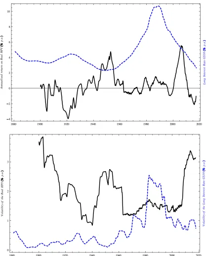
The ad hoc measures taken to resolve the subprime crisis involved expending financial resources to bail out banks without addressing the wave of foreclosures. These short-term amendments negate parts of mortgage contracts and question the disciplining mechanism of finance (Roubini et al. (2009)). Moreover, the increase in volatility of house prices in recent years (see Figure 1) exacerbated the crisis. In contrast to ad hoc approaches, we propose a mortgage contract, the Continuous Workout Mortgage (CWM), which is robust to downturns. We demonstrate how CWMs can be offered to homeowners as anex ante

solution to non-anticipated real estate price declines.

The Continuous Workout Mortgage (CWM, Shiller (2008b)) is a two-in-one product: a fixed rate home loan coupled with negative equity insurance. More importantly its pay-ments are linked to home prices and adjusted downward when necessary to prevent neg-ative equity. CWMs eliminate the expensive workout of defaulting on a plain vanilla mortgage. This subsequently reduces the risk exposure of financial institutions and thus the government to bailouts. CWMs share the price risk of a home with the lender and thus provide automatic adjustments for changes in home prices. This feature eliminates the rational incentive to exercise the costly option to default which is embedded in the loan contract. Despite sharing the underlying risk, the lender continues to receive an un-interrupted stream of monthly payments. Moreover, this can occur without multiple and costly negotiations.

house-1880 1900 1920 1940 1960 1980 2000 2020 4 2 0 2 4 6 8 10 An n ua lis ed re tu rn on Re al H PI p .a . L ong Inte re st Ra te G S10 p .a .

1880 1900 1920 1940 1960 1980 2000 2020

0 1 2 3 Vo la tili ty of the Re al H PI p .a . Vo la tili ty of the L ong Int ere st R ate G S10 p .a .

holds all at once. Households need to proactively plan ahead to mitigate the impact of catastrophic events with low probability as their impact on society can be devastating. Hyman Minsky (1992) emphasizes how the fragility of the financial system culminates in financial/banking crises. Furthermore, real estate crises are correlated with these fi-nancial crises (Piazzesi and Schneider,2016) and exact a huge toll on the macroeconomy by decreasing the GDP (Renaud, 2003; Hoshi and Kashyap,2004). These losses occurred because measures taken, such as deposit insurance, exacerbated banking crises instead of mitigating them (Demirgüç-Kunt and Detrajiache,2002).

Prior to the current crisis, mortgages with repayment schedules contingent on house prices had not been considered. The academic literature, with the exception ofAmbrose and Buttimer(2012), has not discussed their mechanics and especially their design. Shiller is the first researcher, who forcefully articulates the exigency of their employment. CWMs were conceived in1(Shiller(2008b) andShiller(2009)) as an extension of the well-known Price-Level Adjusted Mortgages (PLAMs), where the mortgage contract adjusts to a nar-row index of local home prices instead of a broad index of consumer prices. In their recent study,Ambrose and Buttimer(2012) numerically investigate the properties of Adjustable Balance Mortgages which bear many similarities to CWMs. Alternatively, Duarte and McManus(2011) suggest creation of derivative instruments written on credit losses of a reference mortgage pool. The model inShiller et al.(2013) complements the more intricate one ofAmbrose and Buttimer(2012). Unlike a numerical grid, it relies on a methodology which allows valuation of optional continuous flows in closed form (see e.g. Carr et al. (2000) andShackleton and Wojakowski(2007)).

This paper proposes a solution that makes the housing finance system more robust to shocks through the employment of CWMs. The cost of the insurance stemming from the embedded put option in the CWM is quite low. This is due to economies of scale enjoyed by the lender through: (i) hedging by geographic diversification or resorting to futures contracts; and (ii) proactively underwriting CWMs by making the standards more strin-gent instead of lowering them after a huge run-up in home prices. The second technique is endorsed in Minsky (1992) and Demyanyk and Van Hemert(2011). If financial insti-tutions are able to save the cost of insurance for rare calamities over several real estate cycles, i.e. invest in a fund not correlated with real estate to support higher capital re-serves, it will prevent them from being dependent on taxpayers and government to bail

them out in crisis (as with deposit insurance).

Continuous workout mortgages need markets and indicators for home prices.2 These markets and instruments already exist for lenders to hedge risks. The Chicago Mercantile Exchange (CME) for example, offers options and futures on single-family home prices. Furthermore, reduction of moral hazard incentives requires inclusion of the home-price index of the neighborhood into a repayment formula. This is to prevent moral hazard stemming from an individual failing to maintain or, worse, damaging the property in order to reduce mortgage payments.

Finally, we observe evidence showing the change in retirement trends (seeShiller(2014)). More people are planning to sell their house to consume the proceeds in retirement. No-tably, the continuing care retirement community (CCRC) is a concept that is growing rapidly around the world. However, as a result of the drop in home prices there is a CCRC crisis in the US today and they have a lot of vacancies. If CWMs had existed, they could have helped to insure house values, thus preserve the welfare gain, and immunize retirement consumption from downside variations in the house price index.

In our approach, the homeowner can choose from a classic 30-year Fixed Rate Mortgage (FRM) or an CWM. We show that, for many households, Continuous Workout Mortgages could be a better form of home financing instrument than FRMs.

The next section describes the contracts: the standard Fixed Rate Mortgage and the Con-tinuous Workout contract. In Section3 we extend our closed form approach to include prepayments and defaults. In Section 4 we compute the equilibrium contract rates, the embedded options to default and we assess the impact of prepayment risk. Section 5

describes data and deals with calibration of house price index paths. In Section 6 we then conduct our simulations to numerically compare the expected utilities of Continu-ous Workout and Fixed Rate contracts. Section7concludes. Longer mathematical proofs and the floor flow option formula are collected in AppendicesAandB, respectively.

2_{In a more general case not considered here CWMs could be made dependent on the levels of individual}

2

The contracts

2.1

The standard Fixed Rate Mortgage (FRM)

A major invention introduced during years of Great Depression werefully amortizing re-payment mortgages. Typically, these mortgages are analysed in aT =30 year time hori-zon. For our purposes we use a continuous time representation. In place of the monthly payment we introduce a repayment flow rateRFRMwhich is constant in time. Because in-terest rates have low volatility and are at their historical lows (see Figure1), we motivate prepayments as unpredictable stochastic shocks. Consequently, rates for all maturities are constant and equal tor (see section3 where we extend our setup to include prepay-ment and default risks). To achieve full repayprepay-ment, the mortgage balance Q decreases and becomes zero at maturity. The mortgage balance is equal to the amount owed to the lender at timetand can be computed as the present value of remaining payments

Q RFRM,t =

Z T

t e

r(s t)

RFRM ds = R

FRM

r 1 e

r(T t)

. (1)

Differentiating (1) with respect totwe obtain the dynamics ofQ

dQ

dt = R

FRM_e r(T t) _{= R}FRM

1 rQ

RFRM =rQ R

FRM

. (2)

and the discount rater. The initial equilibrium conditionQ0 =Q RFRM, 0 gives

RFRM = Q0

A(r,T) , (3)

where A(r,T)is the annuity

A(r,T) =

Z T

0 e

rt_{dt =} 1 e rT

r , (4)

i.e. the present value at raterof a unit flow terminating afterTyears.

The simplicity of the FRM becomes problematic when a house develops negative equity. This was the case of many households in the US in years following the burst of the hous-ing bubble in 2007. This is illustrated on Figure2. A $ 500 000 property is financed for 30 years and interest rates are 5%. However, a sharp price decline puts the house in negative equity. House values are well below the line representing the balance. In this example, although the balance in an FRM is set to be fully repaid at maturity, the house is underwa-ter until year 11. In this example the return on original house price is then again negative around year 20 and then year 28, because the value of the property is again below the initial purchase price H0. However, as most of the initial balance have been repaid, the

house is not in negative equity by that time.

2.2

The repayment Continuous Workout Mortgage (CWM)

In this section we argue that a standard repayment FRM can be improved by reducing repayments in bad times. This is illustrated on Figure 3. In this example the household benefits from a substantial reduction, proportional to the drop in the house price, up until year 11 and then again repayments are marginally reduced in years 20 and 28.

For our framework we need a house price index ξ_t which is available for all t 2 [0,T]

and, without loss of generality, an index which is normalized to one initially, i.e.ξ₀ = 1.

0 5 10 15 20 25 30 0

200 000 400 000 600 000 800 000

Time years

R

e

mai

ni

ng

B

al

an

ce

FRM

Home Price

Initial Price

Figure 2: Financing a $500000 property for 30 years with a Fixed Rate Mortgage (FRM) when interest rates are 5%. The drop in home prices puts the house innegative equity.

0 5 10 15 20 25 30

0 5000 10 000 15 000 20 000 25 000 30 000

Time years

Mon

thl

y

pa

yme

nt

CWM

FRM

as

ξ_t = HPIt

HPI0

=₎ Ht =H0ξ_t. (5)

That is, for a house initially worth H0, the quantity H0ξt is aproxy for the value of the house at timet >0.

In good times, when house prices are high, the CWM behaves identically to an FRM. Annual repayments proceed at the maximal annual rate equal to ¯RCW M.3 In bad times, the repayment flow RCW M(ξt) of a Continuous Workout Mortgage (CWM) depends on the house price index and becomes lower than ¯RCW M. It decreases when the house price indexξ_t decreases

RCW M(ξt) = R¯CW Mminf1,ξtg =R¯CW M h

1 (1 ξt)+ i

. (6)

Akin to theconstant annual repayment rate RFRM of an FRM, themaximalannual repay-ment rate ¯RCW M of a CWM is an endogenous parameter (see Figure 4), which must be specified upon origination of the mortgage contract.

When ξ_t < 1 the return on initial housing purchase is negative and the mortgage risks

negative equity if the decline in value is higher than funds repaid so far. In the highly un-likely but not impossible, limiting scenario, when the house price index drops very close to zeroξt !0, the CWM contract automatically produces a full workout i.e.RCW M(ξt) ! 0. That is, the lender absorbs all losses for as long asξt remains close to this lower bound. This can be inferred from the shape of the payoff function illustrated on Figure4. If the collateral becomes worthless, the homeowner should be fully compensated and shouldn’t pay any interest or repay any principal. In other words there is full insurance against house price declines. In more realistic, intermediate situations when the price declines but not by too much, this contract still provides automatic compensation to homeowners. Repayments of principal and the interest are reduced proportionally to the index. As a consequence it is no longer possible to express the current balance as a function of future payments. In fact, for CWMs, (1) no longer holds. Two quantities emerge which will almost surely deviate whent>0:

3_{In our notation we use a ‘bar’ over the letterRto remind us thatR}CW M₍

ξ)cannot become greater than

¯

1. The actual (random) balance to date, which is equal to the present value of the initial balance minus payments done so far

QCW M_t =Q0ert

Z t

0 R

CW M₍

ξ_s)er(t s)ds; (7)

2. The expected payments to occur in future

QCW M_t + =Et Z T

t R

CW M₍

ξs)e r(s t)ds . (8)

The balance QCW M_t is a path-dependent quantity because it is based on past values of the house price index. It can go up as well as down, reflecting the history_fξsgts=0of the

house values observed up to timet. If we know this history we can compute the balance as

QCW M_t =hQ0 R¯CW MA(r,t)

i

ert+R¯CW M

Z t

0

(1 ξs)+er(t s)ds. (9)

In particular we note that h

Q0 R¯CW MA(r,t)

i

ert QCW M_t Q0ert, (10)

so for ¯RCW M > RFRM the lower bound can become negative whent _! T(see Appendix

A.1). This occurs when home prices remained high, the workout did not kick in, the loan fraction of the package was repaid earlier and the mortgagee collected the insurance premium over the lifetime of the contract. However, following a sharp decline in house prices the balance can exponentially increase, as shown by the upper bound. Because payments must stop at maturity, the lender bears risk which he was paid to hold. The borrower has been paying a premium to compensate for this shortfall risk.

Repayments under the CWM contract vary randomly with house prices. The expected payments quantity QCW M_t + should therefore be used for valuation purposes as they re-flect the reality a borrower is facing at a given point in time. It also has the advantage of being forward looking, and thus not path-dependent. However, for computations, we need to assume some distribution of the future value of the indexξ_s : s >t. Historically,

dis-tributed (see e.g.Kau et al.(1985), Kau et al.(1992), Azevedo-Pereira et al. (2003),Sharp et al.(2008),Ambrose and Buttimer(2012)) and here we subscribe to this trend.

At origination t = 0, we require that the initial balance and the expected payments are equal

Q₀CW M =Q₀CW M+ =Q0. (11)

This equilibrium condition is necessary to compute the endogenous repayment flow ¯RCW M

of a CWM. Subsequently, the fair value of theinsurance premia, such as ¯RCW M RFRM em-bedded in a CWM, can also be obtained as well as the CWM and FRMequilibrium contract rates(see Section4).

Proposition 1 The expected present value of future payments of the Continuous Workout Mort-gage (CWM) at time t₂ [0,T]is equal to

QCW M_t + =R¯CW M[A(r,T t) P(ξt, 1,T t,r,δ,σ)] . (12)

where P 0is thefloor(i.e. collection of put options for all maturities from t= 0to t = T) on continuous flowξtcapped at1, expressed in closed form (see AppendixB), andδ,σare the service

flow and the volatility of the house price.

Proof. See AppendixA.2.

The payment flow ¯RCW M which appears in (12) is a constant parameter which is com-puted at origination (t = 0) for the duration of the contract. It should not be confused with the mortgage payment RCW M(ξ_t)given by equation (6) which is a function of

ran-domly changing adjusted house price level ξ_t. Mortgage payments RCW M(ξ_t) decrease

when home prices decline, whilst ¯RCW M is fixed ex ante.

Proposition 2 The repayment flow of a CWM is capped by R¯CW M, which is an endogenous parameter and can be computed explicitly as

¯

RCW M = Q0

A(r,T) P(1, 1,T,r,δ,σ) > R

FRM _{. (13)}

Proof. Sett=0 in (12) and solve for ¯RCW M. Inequality obtains becauseP(1, 1,T,r,δ,σ)>

The endogenous parameter ¯RCW M provides the cap on repayment flow under CWM. Clearly, if the mortgage is fairly priced, parameter ¯RCW M must be greater than RFRM

because the issuer of the insurance must be rewarded. We can think of the difference ¯

RCW M RFRM > 0 as equal to the price of the insurance to be paid in good states of na-ture for the continuous workouts to be automatically provided should bad states occur. If there were no risk to be compensated for (σ ! 0), the present value of insurance puts

represented by the floor function P would become zero and ¯RCW M would equal RFRM. This is illustrated on Figure 5, where we also consider the case of a partial guarantee which only coversα = 1₂ of the loss. Equation (13) is paramount for potential originators

of continuous workouts with repayment features. This pricing condition helps in eval-uating the maximal annual payment for this mortgage. A broker can instantly compute this quantity on a computer screen and make an offer to a customer. Finally, a current estimate could be used and a regulator could mandate an upper bound on volatilityσ.

Furthermore, for an “in-progress” CWM mortgage (at time t > 0), it is interesting to analyse whether its expected present value of future payments is lower or higher than the balanceQ_tFRMof an otherwise identical, standard 30-year FRM. Using (1) and (4) the latter can be written as

QFRMt =Q RFRM,t =Q0A

(r,T t)

A(r,T) . (14)

Similarly, using (12) and (13) we can represent the expected payments of a CWM as

QCW M_t + =Q0

A(r,T t) P(ξt, 1,T t,r,δ,σ)

A(r,T) P(1, 1,T,r,δ,σ) . (15)

Clearly, when house prices are lowξt <1 andtis relatively low we must haveQCW Mt +

QFRM_t . This is because the insurance pays off. However, when house prices are high

ξ_t > 1 and closer to maturity t ! T, we should expect a reversal QCW M_t + QFRM_t . In

this case the insurance puts expire out of the money but a CWM homeowner still has to pay the insurance premia, which results in a slightly higher remaining balance. However, even for very high values of the home price index, expected paymentsQCW M_t +are always capped from above by

¯

QCW Mt =Q0

A(r,T t)

A(r,T) P(1, 1,T,r,δ,σ) Q

CW M+

0 1 2

RCWM

RFRM

RIO

t

R

C

WM

t

CWM annual payment

FRM annual payment

interest only mortgage

Figure 4: Continuous Workout Mortgage (CWM): The repayment flow RCW M(ξt) as a function of the house price indexξ_t.

0.00 0.05 0.10 0.15 0.20 0.25 0.30

10.0 10.5 11.0 11.5 12.0 12.5 13.0

volatility

R

CWM

r 10

CWM , 1

CWM , 1

2

FRM , 0

Figure 5: Maximal CWM payment ¯RCW M as a function of risk σ. Full workout (CWM, α =1, thick line), reduced workout (CWM,α = 1₂,dashed line), no workout (FRM,α =0,

thin line). Riskless rater = 10%, maturityT =30 years, service flow rateδ =4%. Note:

which has been computed as limξ!∞Q

CW M+

t . Note that ¯QCW Mt and QFRMt are similarly shaped, concave functions of time t, both decreasing to zero at maturity T. However,

¯

QCW M_t always dominates QFRM_t . The difference ¯QCW M_t Q_tFRM > 0 is relatively small and represents a “cushion” area above the standard repayment schedule QFRM_t . It is in this area where the insurance premium is collected in good times.

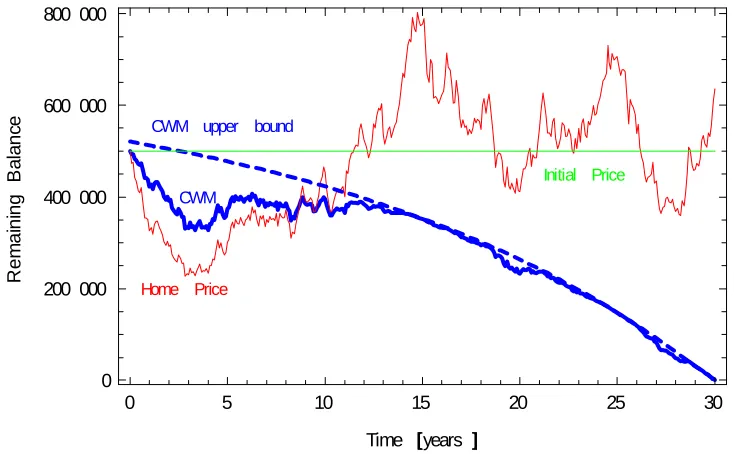
Figures6and7summarize the key differences between FRM and CWM. For FRMs, there is a fixed repayment schedule. In contrast, the repayment schedule for a CWM has a

fixed upper bound. This upper bound is above (but very close to) the FRM’s schedule, forming a “cushion” (see Figure6). The area immediately below the upper bound ¯QCW M_t

(the “cushion”) will get quickly “populated” by QCW M_t + in good times. With reference to FRMs we could therefore say that this extra cushion needs to be there for CWMs to collect the insurance premia in good times. However, in bad times, the CWM’s payments outstanding can dive well below FRM’s outstanding balance (which is fixed for a given time t). This self adjustment mechanism is key to remain away from negative equity, avoid the house becoming underwater and prevent foreclosures automatically (see Figure

7).

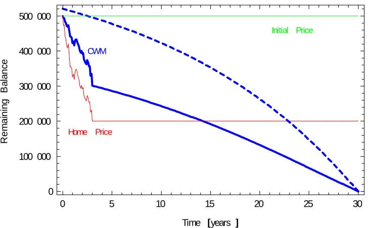
We also investigate the behaviour of a CWM under alternative path scenarios. In the first scenario (Figure8) prices drop and stay at 40% of initial value until maturity. In the second scenario (Figure9) prices also drop to 40% of initial value but then jump and stay at $600000 which represents 110% of the initial value. In both cases expected payments evolve similarly, progressively decreasing to zero at maturity. Obviously, the starting point QCW M_t + for the second scenario is much higher than for the first. However, this starting point must always lie below the upper bound ¯QCW M_t , no matter how much prices appreciate in future.

3

Prepayments and Defaults

0 5 10 15 20 25 30 0

200 000 400 000 600 000 800 000

Time years

R

e

mai

ni

ng

B

al

an

ce CWM upper bound

FRM

Home Price

Figure 6: The CWM’s upper bound on expected future payments v.s. FRM’s scheduled remaining balance.

0 5 10 15 20 25 30

0 200 000 400 000 600 000 800 000

Time years

R

em

ai

ni

ng

B

al

an

ce CWM upper bound

CWM

Home Price

Initial Price

Figure 7: Expected future payments of a CWM,QCW M_t +, as a function of the current house price levels measured by a Home Price indexξ_t and Initial Price H0. The dashed line is

0 5 10 15 20 25 30 0

100 000 200 000 300 000 400 000 500 000

Time years

R

em

ai

nin

g

B

al

an

ce

CWM upper bound

CWM

Home Price

Initial Price

Figure 8: The expected future payments of a CWM when house prices decrease to 40% of initial value and then remain at this level until term.

0 5 10 15 20 25 30

0 100 000 200 000 300 000 400 000 500 000 600 000

Time years

R

em

ai

ni

ng

B

al

an

ce _{CWM CWM upper bound}

Home Price

Initial Price

3.1

Prepayments

In the traditional approach to pricing prepayments non-constant interest rates and their effect on prepayment is examined. In particular, the rational early exercise of the Ameri-can-style prepayment option embedded in a mortgage contract. Modelling these require sophisticated techniques for numerically solving an options pricing problem. In a well-known study Fama (1990) highlights the influence of monetary policy on the behavior of interest rates and thus term structure. It follows that, in the current economic envi-ronment, the prevailing view is that the yield curve will continue to flatten and that the Federal Reserve Board will not raise interest rates drastically. This is elaborated, for ex-ample, in the following recent articles:

“As for skyrocketing long rates, that seems unlikely during the current economic cycle. [...] Since inflation is tamed when real rates rise enough to choke off economic expansion, the lower is the nominal rate necessary to restrain it.”

“Rates are unlikely to skyrocket, despite pundits predictions” ScottMinerd, FT, July 18, 2017, p. 28 “Another month, another impressively low unemployment number, but another flaccid inflation print. No wonder the US Federal Reserve is baffled. Modern macro-economic theory depends upon the famous Phillips curve, and its pressure cooker model of the inflationary process. Let the economy run too hot, and inflation is sure to follow. Let the pressure drop too low, and wage and price growth will ease. Yet in the US, unemployment is at multiyear lows but inflation is nowhere in sight. In the UK it is hardly better. In Japan it is even worse. Across the developed economies, the Phillips curve has gone ignominiously flat. The world’s central bankers are scratching their heads.”

“Lessons from inflation theorists of the past” FelixMartin, FT, July 28, 2017, p. 11

3.1.1 FRM

Let τ be the random refinancing time and 1t<τ the indicator function equal to 1 if

pre-payment did not occur at timetand 0 otherwise. Conditional on prepayment not having occurred before timet 0, the balance of a fully amortizing FRM mortgage should satisfy

ˆ

QFRM_t =E

2 6 6 6 4 Z T

t 1fs<τjt<τge

r(s t)_RFRM_ds

| {z }

payments until τ>t

+ (1+φ)1t<τ Te

r(τ t)_QFRM τ

| {z }

prepayment atτ>t 3 7 7 7

5 , (17)

whereφis the percentage prepayment penalty and the expectationEis to be taken under

the risk-neutral measure. Cash flows are risky, because of the prepayment risk. The outstanding balance at timeτ >tis given by

QFRMτ =

RFRM

r 1 e

r(T τ) _{. (18)}

Working out expectations with respect to the random prepayment timeτ we obtain

ˆ

QFRM_t =

Z T

t F(s)e

r(s t)_RFRM _{ds+ (1+}

φ)

Z T

t h(s)e

r(s t)_QFRM

s ds, (19)

where

F(s) = Eh1_fs<τjt<τgi =Pr(s<τjt <τ) =e λ(s t) (20)

is the cumulative probability of the loan surviving beyond times, conditional on the loan being alive at time t : s > t and λ is the Poisson intensity of the prepayment event.

Similarly, the term h(s) is the conditional probability density of the loan being prepaid within time interval(s,s+ds]i.e.

h(s) = d

ds (1 F(s)) =λe

λ(s t)_{. (21)}

It follows that

ˆ

QFRM_t =

Z T

t e

(r+λ)(s t)_RFRM_{ds+ (1+}

φ)

Z T

t λe

(r+λ)(s t)R

FRM

r 1 e

which gives the following intermediate condition valid fort ₂ [0,T] provided that pre-payment did not occur

ˆ

QFRMt =RFRMx(t) = Q0x (t)

x(0) (23)

where

x(t) = A(r,T t) +φ[A(r,T t) A(r+λ,T t)] (24)

For t = 0 we have ˆQFRM₀ = Q0, which gives the initial equilibrium condition. This

condition can be solved to reveal the fair repayment rate of an FRM, which takes into account subsequent prepayment risk and associated costs

RFRM = Q0

x0

. (25)

where x0 = x(0). We can check that in absence of prepayment risk (λ = 0) or

pre-payment costs (φ = 0) the above formula reverts to (3) which was computed under no

prepayments. We conclude that, from lender’s perspective, a repayment FRM is robust to random prepayments, as long as upon the prepayment event the borrower repays the full amount due, given by (18). The CWM which we study in the next subsection should behave in a similar fashion.

3.1.2 CWM

equal to the loan balance at timet>0

ˆ

QCW M_t =E

2 6 6 6 4 Z T t

1_fs<τjt<τge r(s t)RCW M(ξ_s) ds

| {z }

payments untilτ>t

+ (1+φ)1t<τ Te

r(τ t)_QCW M τ (ξτ)

| {z }

prepayment atτ

3 7 7 7 5 (26)

Here, cash flows are risky, because of the prepayment riskandthe house price risk embed-ded in the house price index ξ. Upon a prepayment event the lender will compute and

inform the borrower about the repayment amount, QCW M_τ (ξ_τ), akin to outstanding balance

of an FRM, to be repaid. Aprepayment penalty is easily added by multiplying the second term by 1+φ, where againφis the percentage penalty. Computed in a fair manner, the

balance at timeτshould take into account the current value of the house price indexξ_τ so

that to reflect the present value of the expected future promised payments of the CWM. That means, unlike for FRMs where annual repayments are insensitive to ξ; e.g. if ξ_τ is

low upon prepayment, the balance to be repaid should be lowered. We already obtained an explicit formula for a fair QCW M_τ (ξ_τ) which should be equal to QCW M_τ +(ξ_τ) given in

equations (12) and (15).

Alternatively, the contract could stipulate the remaining balance as based on the maximal required annual CWM repayment ¯RCW M. This would be similar to an FRM (for which the prepaid amount is based on RFRM), and could be computed using equation (18) where

RFRM should be replaced by ¯RCW M. In any case, the customer should not be required to pay more than ¯RCW M/r(1 exp_f r(T t)_g)plus any prepayment penalty.

Working out expectations with respect to the random prepayment timeτ gives

ˆ

QCW M_t =

Z T

t F(s)e

r(s t)_Eh_RCW M₍

ξ_s)

i

ds+ (1+φ)

Z T

t h(s)e

r(s t)_Eh_QCW M

s (ξs)

i

ds,

(27)

where the expectationEis to be taken along the house price risk dimension represented byξ. The first time integral represents the expected present value of continuous annual

CWM payments RCW M(ξ) received until prepayment date τ or maturity T, whichever

value of the principal outstanding. Using (20), (21) and (27) we obtain

ˆ

QCW M_t = R¯CW M

Z T

t e

(λ+r)(s t)_Eh_{1 (1}

ξs)+ i

ds (28)

+R¯CW M(1+φ)

Z T

t λe

(λ+r)(s t)_{E[[A(r,T s) P(}

ξ_s, 1,T s,r,δ,σ)]]ds.

It is straightforward to compute the first integral, which contains a weighted floor i.e. a weighted time integral of put options. That isλadds to the ratesrandδ

Z T

t e

(r+λ)(s t)_Eh₍₁

ξs)+ i

ds = (29)

=

Z T

t e

(r+λ)(s t)

E

"

1 ξ_texp (r+λ) (δ+λ) σ

2

2 (s t) +σ(Zs Zt)

+#

ds

=P(ξ_t, 1,T t,r+λ,δ+λ,σ) .

This is effectively a weighted sum of floorlets on the normalized house price index ξ

struck at 1 over a continuum of maturities s ₂ [t,T]. Each floorlet is weighted by the probability e λ(s t) _{that the loan will not be prepaid before s > t. By design of the}

contract, in-the-money floorlets (insurance puts) are automatically exercised to lower the annual payment, unless a prepayment happens. Annual payments continue “along” at the rate ¯RCW M until a prepayment happens or maturity is reached. That is, their expected present value must also be adjusted by the prepayment intensity parameterλso that

¯

RCW M

Z T

t e

(r+λ)(s t)_{ds =R}¯CW M_A(r+

λ,T t) . (30)

Integrating the annuity in the second integral is also straightforward

Z T

t e

(r+λ)(s t)_{A(r,T s)ds =} A(r,T t) A(λ,T t)e

r(T t)

r+λ . (31)

A.3)

Z T

t λe

(r+λ)(s t)_E[P(

ξ_s, 1,T s,r,δ,σ)]ds (32)

= P(ξ_t, 1,T t,r,δ,σ) P(ξ_t, 1,T t,r+λ,δ+λ,σ)

We are now ready to state the equilibrium equality that holds at timet 0, determining the equilibrium maximal annual payment ¯RCW Mwhen prepayments occur with intensity

λ. For anyt2 [0,T]andξ_t >0 define the adjusted annuity function

X(ξ_t,t) = A(r,T t) P(ξ_t, 1,T t,r,δ,σ) (33)

+φ A(r,T t) P(ξ_t, 1,T t,r,δ,σ)

A(r+λ,T t) +P(ξ_t, 1,T t,r+λ,δ+λ,σ)

Proposition 3 In presence of prepayments with intensity λ, the value of promised payments of

the CWM at time t>0, with random prepayments included, is equal to

ˆ

QCW M_t + =R¯CW MX(ξt,t) (34)

where X is given by (33). In equilibrium4 QˆCW M_t + = Q0 and (34) can be inverted to derive an estimate5of the equilibrium maximal mortgage paymentR¯CW M

¯

RCW M Q0

X(1, 0) (35)

Remark 4 It is easy to check that under no-prepayments regime (λ! 0), implying A(λ,T) !

T, (35) reduces to (13) from Proposition2. Similarly, in absence of prepayment penalties (φ=0),

(35) simplifies to (13) and (34) reduces to (15). Therefore, from lender’s perspective, the CWM too possesses the “robustness”’ property of the FRM, provided that the prepaid amount is fairly calculated, i.e. (34) is used.

Finally, we note that professional conventions, such as CPR (Conditional Prepayment Rate) and PSA (Public Securities Association) prepayment model, assume that the

pre-4_{For inclusion of arrangement feesπ(points) and default risk and their impact on ¯R}CW M_{see Section4.}

5_{The estimate considered here embeds prepayment risk. See Section4for estimates incorporating both}

payment rate λ is constant in time and independent of the interest rate r. In practice,

however,λwill be influenced by the level of interest rates. FollowingGorovoy and

Linet-sky(2007) we suggest a rate-dependent intensityλ(r)equal to a prepayment intensityλp plus a refinancing intensityλr

λ(r) =λp+λr =λp+l(r r)+ . (36)

The prepayment componentλpaccounts for prepayments due to exogenous reasons such as relocations. The refinancing componentλr increases when the interest raterdecreases. This effect can be calibrated using the multiplierl >0 and the thresholdr >0 parameters. When the interest rater exceeds the thresholdr, the refinancing componentλr vanishes, reflecting the fact that homeowners will not rationally refinance when interest rates are high. Initially, we should haver<r, so that there is no incentive to refinance immediately after the mortgage is originated.

3.2

Defaults

The borrower’s decision to default is more difficult to model. Modelling the endogenous decision to default involves pricing an American put option where the underlying vari-able is the value of the mortgaged property. The standard approach in the literature is to solve the problem using general purpose numerical methods which can be complex to program and time consuming.6

With notable exceptions of the singular perturbation approach ofSharp et al.(2008) and the Viegas and Azevedo-Pereira (2012) Richardson’s extrapolation techniqueà la Geske and Johnson(1984), research for approximate closed-form solutions for mortgages incor-porating the default option have been few. In this section we extend this strand of litera-ture by attaching a default option to our finite-maturity closed-form pricing solution for the CWM we obtained in sections2.2and3.1.

It is well-known from the literature that valuation of American put options is an optimal stopping, free boundary problem, for which no known exact mathematical solution

al-6_{For exampleSharp et al.(2008) report computation times of more than 10 hours for computing just one}

gorithm exists. Consequently, except for very particular cases, not normally encountered in practice, e.g. perpetual mortgages with infinite maturity, there are no closed-form for-mulas available. However, it is incorrect to assume that there is no accurate analytical treatment of options where early exercise is permitted (Shaw,1998, chapter 11). More im-portantly, rushing to numerical methods forces one to abandon quick and efficient com-putation of Greeks by ordinary differentiation. These hedge ratios are involved in the calculation of exposures of Mortgage Backed Securities (MBS). Therefore, this particular aspect is paramount for mortgages and has practical implications for issuers when they manage existing portfolios of MBS or introduce new credit products such as CWMs.

In present context it is important to notice that unlike traded American put options, the underlying house price can only be measured approximately. And, unlike a stock price, it cannot be observed very frequently and the futures series should not be trended. More-over, exogenous factors affect the real magnitude of default options embedded in mort-gages and most of these factors are unobservable and unpredictable. For example, a sud-den loss of income (which is borrower-specific, and thus rarely modeled in the literature) may force a family to default even when house prices are very high. Therefore, the aim here is to have an analytic rather than an accurate or fast valuation,7 to assess how the house price dimension affects the decision to default. Therefore, we will approximate the value of the option to default,D0, by a closed-form approximation.

3.2.1 CWM

We write the value to the lender of the prepayable mortgage,V_tCW M, as equal to

V_tCW M =QCW M_t + Dt QCW M_t +,Ht , (37)

whereQCW M_t +is the expected present value of outstanding payments of a CWM, exposed to prepayments, as given by equation (34) we obtained in the previous section. The sec-ond term on the right hand side, Dt, is the embedded American put option to default. It is a function of the expected outstanding payments QCW M_t +, too, and of Ht, the current value of the property at time t ₂ [0,T]. Below the optimal default threshold HCW M_t the

payoff of the put must satisfy the following free boundary condition8

Dt QCW M_t +,Ht =Q_tCW M+ Ht for allHt HCW Mt and allt (38)

In the default zone the householder saves the expected future payments net of the current value of the house which reverts to the lender via repossession. For what follows it is useful to express QCW M_t + and Ht in terms of the house price index ξ_t we introduced in

Section 3.1 and introduce the corresponding optimal default threshold, ξCW M, for the

index ξ. Lettingξ_t ! ξCW M_t then implies in particular (provided that a prepayment did

not happen beforet) that the optimal exercise boundary, ξCW M_t , of the option to default

can be expressed as

D ξCW M_t ,t =H0 l

ηX ξ

CW M

t ,t ξ

CW M

t for allt, (39)

whereXis given by (33),lis the initial Loan To Value (LTV) ratio

l =Q0/H0 (40)

andη is a normalization parameter, independent oft

η = X(1, 0) . (41)

We have also modified notation of the function D so that to emphasize its dependence on time t and the value of the index ξ_t. Condition (39) is the value-matching condition.

It gives the payoff upon early default. The value of the default option must therefore be equal to the fraction of the initial house price, H0. The scaling factor is an American put

on the house price indexξ_t. Unlike for stock options, the exercise price of this American

put is not constant. It is a function of time t and the index ξt, but also depends on the loan to value ratio l and other parameters embedded in X not shown here, such as the prepayment intensityλ, the prepayment penaltyφ, the volatility of the house price index

σ, etc. For a full list of dependencies see equation (33). From (39) it is also easy to see that

a rational exercise of the default option at origination (t _! 0) would never be optimal when l < 1, i.e. for LTV ratios below 100%, which are typically encountered in practice

8_{In particular, the initial value of the threshold must satisfyH}

0>H0, so that no defaults occur

and never at maturity (t_!T).

The default option must also satisfy the limit condition applicable to any put on underly-ingξ

lim

ξ_t!∞

D(ξt,t) = 0 . (42)

Among all admissible solutions of the partial differential equation obeyed by D satisfy-ing the above condition and all the correspondsatisfy-ing early exercise boundaries ξCW M, we

should retain the solution pairnD,ξCW M

o

which maximizes the value of the default op-tion to the householder. For a given t it can be shown, in a way analogous to Merton (1973) who deals with a simpler case of constant exercise price, that this occurs when the following first order optimality condition, obtained by differentiating (39) with respect to

ξ andlettingξt !ξCW M_t , holds

∂ ∂ξD ξ

CW M

t ,t =H0

l

η ∂ ∂ξX ξ

CW M

t ,t 1 (43)

Note that thissmooth-pastingcondition is substantially different from the standard one for an American put with constant strike, which would just produce H0on the right hand

side. This is because at the point of exercise we have to smoothly paste the default option not into a straight line but into a non-linear strike function, whose curvature depends on time t(as for the FRM) but also (as opposed to the FRM) on the level of the house price indexξ_t.

We can decompose the value of our American putDinto an otherwise identical European default putpplus an early exercise premiumε(see e.g. Carr et al.(1992)), i.e. D = p+ε.

However, for mortgages, unlike for stock options, the value of the default option is always zero at maturity. It follows that p = 0 i.e. the value of the European default put must be zero throughout and D = ε. The value of the put comes entirely from defaulting on

payments before the end of the mortgage i.e. repayment.9

MacMillan (1986) and Barone-Adesi and Whaley(1987) obtain their approximations by

9_{Our approach can still be used for designs where the strike price does not converge to zero at maturity,}

e.g. non amortizing (‘flat’ strike not depending on time or the HPIξ) or partly amortizing mortgages,

considering solutions to the early exercise premiaε(ξ_t,t). In numerous numerical

exper-iments they show that their algorithm is very accurate and considerably more computa-tionally efficient than finite-difference, binomial, or compound-option pricing methods. We adapt their multiplicative separation approach to obtain accurate approximations for our repayment CWM mortgage. In contrast, we can impose separability directly on the function D. We require

D(ξ_t,t) = f (ξ_t) g(t) , (44)

where

g(t) =rA(r,T t) = 1 e r(T t) . (45)

We substitute (44) into the partial differential equation (see (106), AppendixB) obeyed by

D. It follows that

1 2σ

2

ξ2Dξξ+ (r δ)ξDξ+Dt =rD,

where subscripts denote partial derivatives. Substituting (44) and (45) we have

1 2σ

2

ξ2f00(ξ)g(t) + (r δ)ξf0(ξ)g(t) + f(ξ)g0(t) =r f (ξ)g(t) . (46)

Observing g0(t) = re r(T t) = r(g(t) 1), dividing by f (ξ)and g(t) and noting the

function g(t)as if it were a constantg, we obtain

1 2σ

2

ξ2f

00_(ξ)

f (ξ) + (r δ)ξ

f0(ξ)

f (ξ) =

r

g(t) . (47)

This equation is not properly separated because g(t) is not a constant but a function of time t. If g(t) were a constant, i.e. if we could write g(t) = g, the solution to the corresponding ordinary differential equation with constant coefficients would have the form

whereaCW Mis a constant andqis the negative root of the quadratic equation

1 2σ

2_q(q

1) + (r δ)q = r

g(t) , (49)

so that (42) holds. However, becausegis a function of time, so must beq, which gives

q(t) = 1

2 r δ σ2 s 1 2 r δ σ2 2 + r

g(t)

2

σ2 <0 , (50)

whereg(t)is given by (45). It follows that we can express the option to default as

D(ξ,t) = aCW Mξq(t)g(t) , (51)

whereq(t)is given by (50). The constantaCW M and the optimal exercise boundaryξCW M_t

at time t have to be determined from the value-matching (39) and smooth-pasting (43) system of equations

8 > < > :

aCW Mg(t) ξCW M_t

q(t)

= H0

h l

ηX ξ

CW M

t ,t ξ

CW M t

i

aCW Mg(t)q(t) ξCW M_t

q(t) 1 = H0

h l

η ∂ ∂ξX ξ

CW M

t ,t 1

i .

(52)

Dividing side-wise the second equation by the first,aCW M is eliminated and we get

1

q(t) =

1

ξCW M_t

l

ηX ξ

CW M

t ,t ξ

CW M t l

η ∂ ∂ξX ξ

CW M

t ,t 1

, (53)

which can easily be solved numerically to obtain the boundaryξCW M_t . In particular, both

X(ξ,t) and it’s derivative _∂ξ∂ X(ξ,t) are available in closed form.10 OnceξCW M_t is

calcu-lated, aCW M can be obtained from either of the equations of the system (52). This ends the valuation of the embedded default put option (51). We note in particular that the final result, (51), is notmultiplicatively separable in ξ and twhich contradicts the initial

assumption.11 However, the method is atour de forceas it achieves the stated goal, which

10_{Closed form expressions for partials of the floor} ∂

∂ξP(ξ, 1,T t,r+λ,δ+λ,σ)can be found in Shack-leton and Wojakowski(2007). For computations, sinceX(ξ,t)is given in closed form (33), we used Mathe-maticacomputer algebra software to calculate these partials in closed form.

11_{Dis of the form f(}

is to obtain accurate values ofboththe option and the free boundary.

Finally, we note that, thelogarithmof the final result is multiplicatively separable inξ and

t. That is, we have lnD = ϕ(ξ) χ(t)where ϕ,χare some functions. Note that if instead

we had the initial assumption satisfied all along, i.e. D = f (ξ) g(t), theBarone-Adesi

and Whaley(1987) method would be an exact method for pricing American options and not an approximation.

3.2.2 FRM

The value to the lender of a prepayable, fixed rate mortgage, V_tFRM, can also be decom-posed into

VtFRM = QˆFRMt DtFRM QˆFRMt ,Ht , (54)

where ˆQFRM_t is the expected present value of outstanding payments of an FRM, subject to prepayments, as given by equation (23) we obtained in the previous section. Function

DFRM_t , is similarly, the embedded American put to default. Below the optimal default threshold H_tFRM, which will be different from HCW M_t , must satisfy the initial condition

HFRM_t < H0too and the free boundary condition

DFRM QˆFRM_t ,Ht =QˆFRMt Ht for allHt HFRMt and allt (55)

Borrower maximizes value by defaulting immediately after crossing down the boundary

HFRM_t . Using (23) and (5) gives

DFRM QˆFRMt ,Ht =Q0x (t)

x0 H0ξt , (56)

where x0 = x(0)and x(t) is given by (24). Using notationl = Q0/H0for the LTV ratio

as before, rearranging, letting ξ_t ! ξ_tFRM and conditional on prepayment not

happen-ing before t 0, the default option can be written as a function of the optimal exercise boundary,ξ_tFRM

DFRM ξFRM_t ,t = H0 l x0x

Condition (57) is thevalue-matchingcondition for an FRM and gives the payoff upon early default, a fraction of the initial house price,H0. The exercise price of the scaling American

put on the house price indexξ_t is here a function of timet, loan to value ratioland early

prepayment parameters (intensity λand penaltyφ) but is not a function of the indexξ_t

or its volatilityσ.12 This is why thesmooth-pastingcondition for FRM here is analogue to

a standard American put, where the strike does not depend on the underlying asset, and simplifies to

∂ ∂ξ_tD

FRM

ξ_tFRM,t = H0 (58)

We decompose DFRM into a European put plus an early default premium: DFRM =

pFRM+εFRM and notice that pFRM = 0. At maturity the loan is fully amortized and

default is impossible, implying DFRM = εFRM. We then follow the Barone-Adesi and

Whaley(1987) andMacMillan(1986) as we did for the CWM. We impose separability

DFRM(ξ_t,t) = fFRM(ξ_t) g(t) , (59)

where g(t) is given by (45), the same as for the CWM. We substitute (59) into the partial differential equation (see again (106), Appendix B) obeyed by DFRM to discover that it follows that same Partial Differential Equation asDCW Mand must have the same form of the power solution

DFRM(ξ,t) = aFRMξq(t)g(t) (60)

where q(t) is the same, negative solution of the fundamental quadratic, given by (50) and aFRM is a constant proper to an FRM which must be calculated from the system of two equations derived from the value-matching (57) and smooth-pasting (58) boundary conditions

8 > < > :

ξFRM_t

q(t)

aFRMg(t) = H0 _xl₀x(t) ξ_tFRM

aFRMq(t) ξFRM_t

q(t) 1

g(t) = H0.

(61)

12_{Here too a rational default at origination (t!0) or maturity (t!T) would never be optimal for LTV}

ratios below 100% (l<1). Similarly limξt!∞D

CW M_(ξ

EliminatingaFRMwe get

ξ_tFRM =

lx_x(t) 0

1 _q(1_t)

Interestingly this reveals that the (approximate) boundaryξFRM_t can be obtained inclosed

formand so can the default option “scale,” the constantaFRM

aFRM = H0

g(t)q(t) ξ

FRM t

1 q(t)

= H0

g(t)q(t) 0 @ l

x(t) x0

1 _q(1_t) 1 A

1 q(t)

(62)

which gives thedefault option for FRM in closed form

DFRM(ξ,t) = H0

q(t) 0 @ l

x(t) x0

1 _q(1_t) 1 A

1 q(t)

ξq(t) (63)

Finally note that although not explicit in our notation,x(t)and x0do depend on

prepay-ment frequency and penalty parametersλ,φ(see equation (24)).

4

Equilibrium contract rate for the CWM and the FRM when

default and prepayment risks are present

The point of our paper is that the FRM and the CWM have different risks embedded in them. The FRM places house price risk entirely on the borrower until the point where they would default. The CWM mitigates this risk and, depending on design of how the repayment schedule responds to changes in house prices, transfers all or considerable portions of the house price risk to the lender. The lender is paid a risk premium, in the form of increased repayment rates of the CWM in good states, to bear this risk.

and the default risk premia in the value of a CWM to the lender (see equation (37)). Using Black Scholes options pricing framework these premia can be computed as expectations under the martingale measure of the expected future CWM and FRM payoffs, discounted using the riskless rate r. As a result, both CWM and FRM are correctly priced, even though pricing by arbitrage requires discounting using the same rate.

We initially expressed ourequilibriumresult in the language ofequilibrium annual payments,

RFRM and ¯RCW M (and to be more precise: equilibrium annualmaximal payment ¯RCW M, in the case of the CWM). We will now establish a link between these quantities and the equilibrium contract rates for the CWM and the FRM.

4.1

FRM

For a mortgage with initial balanceQ0the monthly compounded ‘contract rate’ ¯rcis typi-cally defined via the equation linking the maturityN(expressed as the number of months remaining) and the monthly paymentMP

Q0 = MP

¯

rc

12

1 1

1+ ¯rc

12

N !

(64)

It is expressed in percentages per annum and is discretely compounded. Clearly, if all the monthly payments MPare riskless, the right hand side is the present value of a monthly paid annuity and ¯rcmust be equal to the riskless rate. This definition is still used in pricing situations where spot riskless rates are stochastic and monthly payments are implicitly

stochastic i.e. where the monthly paymentMPcan randomly discontinue before maturity due to prepayment or default, see e.g.Kau et al.(1992). In these papers, for a given initial balanceQ0, term Nand a candidate solution contract rate rc the corresponding monthly ‘promised’ paymentMPis computed via equation (64). It is then checked by solving the pricing PDE numerically (Feynman-Kac), whether the present value (discounted at the riskless rater) of risk-neutral expectations of the series of monthly paymentsMPis equal toQ0. If it is, that means the rate ¯rc is the equilibrium contract rate.

continuous-time expression, analogous to (64)

Q0 = R

FRM

rFRMc

1 expn rcFRMT o

(65)

whererFRM_c is the equilibrium, continuously compounded FRM contract rate, expressed in percentages per annum. This means that knowing the equilibrium annual repayment rateRFRM, we can figure out the correspondingequilibrium FRM contract rate r_cFRM. When all FRM cash flows are riskless, we must have rFRM_c = r, where r is the riskless rate. To avoid the contractual arbitrage, the equilibrium condition which must be satisfied at origination is

Q0(1 π) =V₀FRM =Qˆ₀FRM DFRM(1, 0) (66)

That is, the valueQ0of the home loan granted by the lender minus anyarrangement fees

π(points) expressed as a percentage of the loan, should be equal to the value of the

mort-gage to the lender, i.e. the value of promised payments, considering the possibility of prepayment, minus the option to default. This gives13

H0l(1 π) = RFRMx0+ H0

q0 l

1 _q1

0

!1 q0

(67)

which we can solve for the (promised) annual repayment rateRFRM

RFRM = H0

x0

2

4l(1 π) 1

q0 l

1 _q1

0

!1 q03

5 (68)

and obtain the continuously compounded equilibrium contract rate rFRM_c by inverting (65). It turns out that this, again, can be obtained in closed from

rcFRM = 1

T

RFRMT Q0

+W R

FRM_T

Q0 exp

RFRMT

Q0 , (69)

whereW is theLambert-Wfunction, also known asproduct log. BecauserFRM_c is a

¯

rFRM_c [%]

T = 15 20 25 30

σ =5%

Intensity + BAW 10.124 10.112 10.105 6.026 PDE 10.146 10.124 10.146

Binomial 5.134

σ =10%

Intensity + BAW 10.597 10.523 10.478 6.224 PDE 10.028 10.082 10.113

Binomial 6.22

Table 1: A quick comparison of equilibrium contract rates. Intensity + BAW: this work; PDE: Crank-Nicolson PSOR approach of Sharp et al. (2008) r = r0 = 10%, δ = 7.5%;

Binomial: twin-tree approach ofAmbrose and Buttimer(2012)r =6%,r0 =4%,δ=2%.

ously compounded rate, it can be converted to monthly rate via

¯

rcFRM =12 exp 1 12r

FRM

c 1 . (70)

We start by checking the output of our model against figures obtained using other meth-ods. From Table1it emerges that, when house price volatility is small, our approximate contract rates tend to slightly undervalue the allegedly very high accurate PDE solutions obtained viaCrank and Nicolson (1947) implicit PSOR scheme approach of Sharp et al. (2008). When volatility is high the opposite happens. Our estimates also slightly over-value the Binomial approach of Ambrose and Buttimer (2012), but are very close for

σ = 10%. However this is less surprising as their term structure is steep (spot rate r

starts at 4% and converges to 6% in long term) while the term structure of Sharp et al. (2008) is flat (spot raterstarts at 10% and remains in the vicinity of 10% in the long term). Consistently with the options pricing theory, the higher the volatility of the house price, the higher the equilibrium contract rates obtained from our model. Also consistently with common wisdom (and unlike the PDE results ofSharp et al.(2008) which exhibit a local minimum at T = 20 years), the longer the term of the mortgage contract, the lower our model’s equilibrium mortgage rates.14

14_{Sharp et al.(2008) work from European perspective with maturities typically up to T = 25 years in}

the UK whileAmbrose and Buttimer(2012) work with the standard T = 30 year maturity US mortgage. We only report contract values for lowest volatilities of interest rate they consider i.e. forσr =5%. This is

4.2

CWM

In contrast, because cash flows of the CWM are explicitly stochastic, defining the corre-sponding ‘contract rate’ is not straightforward. However, by analogy with (64) and (65) we posit

Q0 =

¯

RCW M rCW Mc

1 expn rCW Mc T o

(71)

where ¯RCW M is theequilibrium annual repayment rate of the CWM (which we obtained in closed form) and rCW Mc is the corresponding equilibrium CWM contract rate. Because CWM cash flows are all stochastic and capped by ¯RCW M, which is the equilibriummaximal

annual repayment rate, rCW M_c is in fact the equilibrium CWM maximalcontract rate. To obtain ¯RCW M we start with the same initial equilibrium condition as we were using for FRM

Q0(1 π) =V0CW M =QˆCW M0 DCW M(1, 0) (72)

where V₀CW M is the value to the lender andπ are the points. The major difference is the

DCW M(1, 0) component which is in closed form too but requires one of the arguments (the early default boundaryξCW M₀ ) to be solved for numerically. Using (34) we obtain

¯

RCW M = Q0(1 π) +D

CW M_{(1, 0)}

X(1, 0) (73)

which in conjunction with (71) should be used to obtain the CWM contract rate rCW M_c . Monthly compounded CWM contract rate is obtained fromrCW M_c using

¯

rCW M_c =12 exp 1 12r

CW M

c 1 . (74)

4.3

CWM v.s. FRM contract rates

RFRM = Q0(1 π) +D

FRM_{(1, 0)}

A(r,T) v.s. R¯

CW M ₌ Q0(1 π) +DCW M(1, 0)

A(r,T) P(1, 1,T,r,δ,σ) (75)

There are two opposite effects which determine the CWM maximal annual payment ¯

RCW M. On one hand CWM commands a positive insurance componentP(1, 1,T,r,δ,σ)

which is subtracted from annuity A(r,T)in the denominator. Thisincreasesthe maximal annual payment ¯RCW M relative to RFRM. On the other hand we expect the value of the embedded option to default, appearing in the numerator, to belowerfor the CWM

DCW M(1, 0) <DFRM(1, 0) (76)

and toreducethe annual payment ¯RCW Mas a result, relative to the FRM.

Our numerical analysis shows that the insurance effect dominates the default option ef-fect. That is, the maximal annual payment of the CWM is above the constant annual payment of the FRM. However, under many scenarios, the decrease in the embedded option to default is sufficiently prominent for the CWM to offer very affordable contract rates which are only slightly higher than the contract rates of an FRM. This shows that at least some part of the costs of the insurance against default can be financed by reducing the incentives to rationally default when house prices decrease.

Payout ratesδreflect service provided by the property but also the speed of its

deprecia-tion relative to the growth of other assets in the economy. Consider a case where interest rates are are low and comparable to the service flow (r = δ = 2%). For the loan to value

ratiol =95% (see Table2) the contract rate of a CWM is only 2.550%, compared to 2.342% for an otherwise identical FRM. When interest rates increase tor =12%, the attractiveness of the CWM is preserved. Contract rates follow the interest rate to 12.063% and 12.061% for the CWM and the FRM, respectively. Meanwhile, their relative spread decreases by two orders of magnitude, from 20.8 to only 0.2 basis points. Decreasing the loan to value ratio tol =90% widens the spread to 0.3 basis points and remains the same forl =80%.

Consistent with option pricing theory, the spread between CWM and FRM loan rates increases as the volatility of the house prices increases. In our example, when the house price volatility increases fromσ=5% to 15% (see Table4), FRM and CWM rates increase

rc mth % p/a σ= 0.05 T= 30. π= 0.

FRM CWM

l r δ none low high none low high

0.95 0.02 0.02 2.342 2.27 1.639 2.55 2.477 1.839 0.06 3.609 3.532 2.855 6.03 5.943 5.165 0.12 4.725 4.642 3.921 12.063 11.944 10.837

0.06 0.02 6.034 5.948 5.169 6.043 5.956 5.178 0.06 6.328 6.24 5.448 6.608 6.518 5.714 0.12 7.94 7.843 6.972 12.071 11.952 10.845

0.12 0.02 12.061 11.942 10.836 12.063 11.944 10.838 0.06 12.068 11.949 10.843 12.076 11.957 10.85 0.12 12.367 12.246 11.12 12.751 12.627 11.478

0.9 0.02 0.02 2.256 2.184 1.556 2.534 2.462 1.824 0.06 3.526 3.449 2.775 6.03 5.943 5.165 0.12 4.666 4.584 3.865 12.063 11.944 10.837

0.06 0.02 6.018 5.932 5.154 6.031 5.944 5.166 0.06 6.229 6.141 5.354 6.603 6.513 5.708 0.12 7.828 7.732 6.867 12.071 11.952 10.845

0.12 0.02 12.06 11.941 10.835 12.063 11.944 10.837 0.06 12.061 11.942 10.836 12.071 11.952 10.845 0.12 12.244 12.124 11.006 12.751 12.627 11.478

0.8 0.02 0.02 2.136 2.065 1.44 2.534 2.462 1.824 0.06 3.358 3.282 2.614 6.03 5.943 5.165 0.12 4.543 4.462 3.748 12.063 11.944 10.837

0.06 0.02 6.015 5.928 5.151 6.03 5.943 5.165 0.06 6.108 6.021 5.239 6.603 6.513 5.708 0.12 7.606 7.511 6.657 12.071 11.952 10.845

0.12 0.02 12.06 11.941 10.835 12.063 11.944 10.837 0.06 12.06 11.941 10.835 12.071 11.952 10.845 0.12 12.121 12.001 10.891 12.751 12.627 11.478

Table 2: Equilibrium contract rates v.s. prepayment intensity and cost. r¯c[%] p.a. monthly compounded. House price volatility σ = 5%, mortgage term T = 30 years,

pointsπ = 0. Prepayment intensity and cost: λ = 0,φ = 0 (none),λ = 1/year,φ = 1%

rc mth % p/a σ= 0.1 T= 30. π= 0.

FRM CWM

l r δ none low high none low high

0.95 0.02 0.02 2.776 2.702 2.056 3.253 3.178 2.514 0.06 3.787 3.709 3.025 6.185 6.098 5.313 0.12 4.793 4.71 3.986 12.097 11.977 10.869

0.06 0.02 6.255 6.167 5.379 6.335 6.247 5.455 0.06 6.765 6.674 5.862 7.358 7.264 6.423 0.12 8.106 8.008 7.128 12.188 12.068 10.954

0.12 0.02 12.145 12.025 10.914 12.163 12.043 10.931 0.06 12.251 12.13 11.012 12.31 12.189 11.068 0.12 12.846 12.721 11.565 13.587 13.458 12.254

0.9 0.02 0.02 2.68 2.606 1.963 3.148 3.073 2.413 0.06 3.707 3.629 2.949 6.185 6.098 5.313 0.12 4.736 4.654 3.932 12.097 11.977 10.869

0.06 0.02 6.166 6.078 5.294 6.254 6.166 5.378 0.06 6.643 6.553 5.746 7.256 7.163 6.327 0.12 7.997 7.9 7.026 12.188 12.068 10.954

0.12 0.02 12.089 11.969 10.862 12.114 11.994 10.885 0.06 12.155 12.035 10.923 12.229 12.109 10.992 0.12 12.677 12.554 11.409 13.503 13.375 12.177

0.8 0.02 0.02 2.509 2.436 1.799 3.119 3.044 2.386 0.06 3.545 3.468 2.794 6.185 6.098 5.313 0.12 4.616 4.535 3.818 12.097 11.977 10.869

0.06 0.02 6.069 5.982 5.203 6.194 6.106 5.321 0.06 6.441 6.352 5.555 7.247 7.154 6.318 0.12 7.779 7.683 6.82 12.188 12.068 10.954

0.12 0.02 12.063 11.944 10.838 12.097 11.978 10.87 0.06 12.081 11.962 10.854 12.19 12.07 10.956 0.12 12.424 12.303 11.174 13.503 13.375 12.177

Table 3: Equilibrium contract rates v.s. prepayment intensity and cost. r¯c[%] p.a. monthly compounded. House price volatility σ = 10%, mortgage term T = 30 years,

pointsπ = 0. Prepayment intensity and cost: λ = 0,φ = 0 (none),λ = 1/year,φ = 1%