Abstract In statistical data analysis by analysis of variance, the

(1)

Abstract—In statistical data analysis by analysis of variance, the usual basic assumptions are that the model is additive and the errors are randomly, independently, and normally distributed about zero mean and constant variance. For analyzing data which do not match the assumptions of the conventional method of analysis, we have two choices. We may transform the data to fit the assumptions, or we may develop new methods of analysis with assumptions which fit the original data. If we can find a satisfactory transformation, it will almost always be easier to use it rather than to develop a new method of analysis. In analysis of variance with Weibull data, the data should first be transformed to fit all the assumptions required. The well-known Box-Cox transformation can use to get the normality but cannot transform the observations that equal zero. In the sets of Weibull data, the observations may be zero. To cope this problem, an alternative transformation is proposed. When the transformed data have met the required assumptions of normality and homogeneity of variances, we then can apply the analysis of variance to test the equality of the population means or the treatment effects of the original Weibull populations. Moreover, numerical studies of the powers of the tests obtained from ANOVA of the transformed data are also given.

Keywords—Weibull Data, The Box-Cox transformation, The alternative transformation

I. INTRODUCTION

In the analysis of variance (ANOVA) the usual basic assumptions are that the model is additive and the errors are randomly, independently, and normally distributed about zero mean and equal variances. With some specific sets of data, the basic assumptions are not satisfied so analysis of variance cannot be applied appropriately. Tukey [1]suggested that in analyzing data which do not match the assumptions of the conventional method of analysis, we have two alternative ways to go about. We may transform the data to fit the assumptions, or we may develop some new methods of analysis with assumptions fitting the original data. If we can find a satisfactory transformation, it will almost always be easier to use the conventional method of analysis rather than to develop a new one. Montgomery [2] suggested that transformations are used for three purposes, stabilizing response variance, making the distribution of the response variable closer to the normal distribution, and improving the fit of model to the data. Choosing an appropriate

This work was supported in part by the Faculty of Science, Maejo University, Chiang Mai, Thailand.

L. Watthanacheewakul is with the Faculty of Science, Maejo University, Chiang Mai, Thailand (phone: 66-53-873-551; fax: 66-53-878-225; e-mail: [email protected]).

transformation depends on the probability distribution of the sample data. For example, the square root transformation is used for Poisson data and the logarithmic transformation is used for lognormal data. Moreover, we can use the

relationship between the standard deviation and the mean for stabilizing variance. Furthermore, we can transform the data by using a family of transformations studied for a long time. Many authors have studied the transformations of the data to meet the requirements of the analysis of variance [3]- [6]. The Box-Cox transformation for ANOVA is in the form

1

, 0

ln , 0 ⎧ −

≠ ⎪

= ⎨

⎪ ₌

⎩

ij

X Y

X

λ

λ λ

λ

for x_ij>0 (1)

where X_ij is a random variable in the j th trial from the i th

distribution,

Y_ij the transformed variable of X_ij, and

λ a transformation parameter. It is often used to transform the data to fulfill the requirements but it might not be satisfactory in some cases. Doksum and Wang [7]indicated that the Box-Cox

transformation should be used with caution in some cases such as failure time and survival data. John and Draper [6] showed that the Box-Cox transformation was not satisfactory even when the best value of transformation parameter have been chosen. Moreover, the condition of observation is that the value of it is greater than zero. In the sets of Weibull data, the some observations may be zero. In order to cope with this problem, the alternative transformation is proposed. In this paper, the two parameter Weibull distribution is investigated.

II. THE WEIBULL DISTRIBUTION

The Weibull distribution is a continuous probability distribution. It is named after Waloddi Weibull who described it in detail in 1951. The probability density function of a two parameter Weibull random variable X is

1

, 0; , 0

( )

0 , <0 − ⎛ ⎞

−⎜ ⎟ ⎝ ⎠

⎧ ⎛ ⎞

⎪ _{⎜ ⎟} _≥ _>

= ⎨ ⎝ ⎠ ⎪ ⎩

x

e x

f x

x

α

α β

α _{α β}

β β ’ (2)

where α is the shape parameter and β is the scale parameter.

Analysis of Variance with Weibull Data

(2)

The mean is ⋅Γ⎛_⎜1+1⎞_⎟

⎝ ⎠

β

α . It’s useful in many fields such as

survival analysis, extreme value theory, weather forecasting, reliability engineering and failure analysis. Moreover, it is used to describe wind speed distribution, the particle size distribution, and so on. Furthermore, it is related to the other probability distribution such as the exponential distribution when α=1 [8]. An alternative test procedure for testing the equality of scale parameters of k Weibull populations with a common shape based on sample quantiles was presented and the power of this procedure was shown to be quite good numerically in several situations [9].

III. AN ALTERNATIVE TRANSFORMATION

A transformation for any sets of Weibull data to normality with equal variances proposed here is in the form

0.01 1

, 0 ln 0.01 , 0 ⎧ ⎡_⎣ + ⎤_⎦ − ⎪ ≠ ⎪ = ⎨ ⎪ ⎡ + ⎤ = ⎪ ⎣ ⎦ ⎩ ij i ij ij i X c Y X c λ λ λ λ (3)

where X_ij is a random variable in the j th trial from the i

th

Weibull distribution,

Y_ij the transformed variable of X_ij,

ci the range of the value of Xijfrom the i th

Weibull distribution, and λ a transformation parameter.

The likelihood function in relation to the observations is given by

2 2

2

2 2 1 1

0.01 1

1 1

( , ) exp . ( ; ),

2

(2 ) = =

⎧ _⎡_⎡ ₊ _⎤ ₋ _⎤⎫

⎪ _⎢⎣ ⎦ _⎥⎪

= ⎨− _⎢ − _⎥⎬

⎪ _⎣ _⎦⎪

⎩ ⎭

∑∑k ni

ij i

i ij n i

i j

X c

L x J x

λ

μ σ μ λ

σ λ πσ (4) where 1 1 ( ; ) = = ∂ = ∂

∏∏

k ni

ij

i j ij

y J y x

x 1 1 0.01 1 = = ⎡_⎡ ₊ _⎤ ₋ ⎤ ∂ ⎣_⎢ ⎦ _⎥ = ⎢ ⎥ ∂ ⎣ ⎦

∏∏

k ni

ij i

i j ij

X c x λ λ 1 1 1 0.01 − = = ⎡ ⎤

=

∏∏

k ni _⎣ ij+ i_⎦

i j

X c λ .

For a fixed λ, the MLE’s for _and 2

i

μ σ are

1 0.01 1 1 ˆ = ⎡ + ⎤ − ⎣ ⎦

=

∑

ni

ij i i j i X c n λ μ

λ (5)

and

2 2

1 1 1

0.01 1 0.01 1

1 1 ˆ . = = = ⎧_⎡ ₊ _⎤ ₋ ⎛_⎡ ₊ _⎤ ₋ ⎞⎫ ⎪⎣ ⎦ ⎜⎣ ⎦ ⎟⎪ = ⎨ − _⎜ _⎟⎬ ⎪ _⎝ _⎠⎪ ⎩ ⎭

∑∑

k ni

∑

ni

ij i ij i

i j i j

X c X c

n n

λ λ

σ

λ λ (6)

Substitute the values of ˆμ_iand _σ_ˆ2_{into the likelihood} equation (4). Thus for fixed λ, except for a constant, the maximized log likelihood is

2

1 1 1

1 1

( ) ln ( )

0.01 1 0.01 1

1 1

ln 2

( 1) ln 0.01

= = = = = = = ⎛ _⎧ _⎡ _⎤_⎫ ⎞ ⎡ + ⎤ − ⎡ + ⎤ − ⎜ ⎪⎣ ⎦ _⎢⎣ ⎦ _⎥⎪ ⎟ − ⎜ ⎨ − _⎢ _⎥⎬ ⎟ ⎪ ⎪ ⎜ _⎩ _⎣ _⎦_⎭ ⎟ ⎝ ⎠ ⎡ ⎤ + − _⎣ + _⎦

∑∑

∑

∑∑

i i i ij n n k

ij i ij i

i j i j

n k

ij i

i j

f L x

X c X c

n n n X c λ λ λ λ λ λ λ (7) Hence, 2 1 1 2 2

1 1 1 1

ln ( )

0.01 ln 0.01

1 0.01 0.01 = = = = = = = ⎡ _⎡ _⎤ _⎡ _⎤⎤ − _⎢ _⎣ + _⎦ _⎣ + _⎦_⎥ ⎣ ⎦ ₊ ⎛ ⎞ ⎡ + ⎤ − _⎜ ⎡ + ⎤ _⎟ ⎣ ⎦ ⎣ ⎦ ⎝ ⎠ ∑∑ ∑∑ ∑ ∑ i i i n k

ij i ij i

i j

n n

k k

ij i ij i

i j i i j

d L d

n X c X c

X c X c

n

λ

λ λ

λ

1 1 1

2 2

1 1 1 1

1 1

1 _0.01 _0.01 _ln _0.01

1 0.01 0.01 ln 0.01 = = = = = = = = = ⎡ ⎛ ⎞⎛ ⎞⎤ ⎡ + ⎤ ⎡ + ⎤ ⎡ + ⎤ ⎢ ⎜ ⎣ ⎦ ⎟⎜ ⎣ ⎦ ⎣ ⎦⎟⎥ ⎢ ⎝ ⎠⎝ ⎠⎥ ⎣ ⎦ ⎛ ⎞ ⎡ + ⎤ − ⎜ ⎡ + ⎤ ⎟ ⎣ ⎦ ⎣ ⎦ ⎝ ⎠ ⎡ ⎤ + + _⎣ + _⎦ ∑ ∑ ∑ ∑∑ ∑ ∑ ∑∑ i i i i i n n k

ij i ij i ij i

i i j j

n n

k k

ij i ij i

i j i i j

n k

ij i

i j

X c X c X c

n n

X c X c

n n X c λ λ λ λ λ (8)

The maximum likelihood estimate of

λ

is obtained by solving the likelihood equation

2

1 1

2 2

1 1 1 1

0.01 ln 0.01

1 0.01 0.01 = = = = = = ⎡ _⎡ _⎤ _⎡ _⎤⎤ − _⎢ _⎣ + _⎦ _⎣ + _⎦_⎥ ⎣ ⎦ ₊ ⎛ ⎞ ⎡ + ⎤ − ⎜ ⎡ + ⎤ ⎟ ⎣ ⎦ _⎝ ⎣ ⎦ _⎠ ∑∑ ∑∑ ∑ ∑ i i i n k

ij i ij i

i j

n n

k k

ij i ij i

i j i i j

n X c X c

X c X c

n

λ

λ λ

1 1 1

2 2

1 1 1 1

1 1

1 _0.01 _0.01 _ln _0.01

1

0.01 0.01

ln 0.01 0

= = = = = = = = = ⎡ ⎛ _⎡ ₊ _⎤ ⎞⎛ _⎡ ₊ _⎤ _⎡ ₊ _⎤⎞⎤ ⎢ ⎜ ⎣ ⎦ ⎟⎜ ⎣ ⎦ ⎣ ⎦⎟⎥ ⎢ ⎝ ⎠⎝ ⎠⎥ ⎣ ⎦ ⎛ ⎞ ⎡ + ⎤ − ⎜ ⎡ + ⎤ ⎟ ⎣ ⎦ _⎝ ⎣ ⎦ _⎠ ⎡ ⎤ + + _⎣ + _⎦= ∑ ∑ ∑ ∑∑ ∑ ∑ ∑∑ i i i i i n n k

ij i ij i ij i

i i j j

n n

k k

ij i ij i

i j i i j

n k

ij i

i j

X c X c X c

n n

X c X c

n n X c λ λ λ λ λ (9)

Since λappears on the exponent of the observations, it is considered to be too complicated for solving it. The

maximized log likelihood function is a unimodal function so the value of the transformation parameter is obtained when the slope of the curvature of the maximized log likelihood function is nearly zero [3]. Hence we can also use the numerical method such as bisection for finding the suitable value of λ.

IV. AN EXAMPLE

(3)

[image:3.595.366.491.86.209.2]

0.8 and the scale parameter is 2,500.The shape parameter of the third population is 0.3 and the scale parameter is 2,800. Supposing that three random samples of size 20 are taken from each Weibull population, the sample data are shown in Table I.

TABLEI

THREE RANDOM SAMPLES OF SIZE 20

TAKEN FROM EACH OF THREE WEIBULL POPULATIONS

Sample 1

Sample Sample 2 3

2579.6908 84.7686 6401.1384

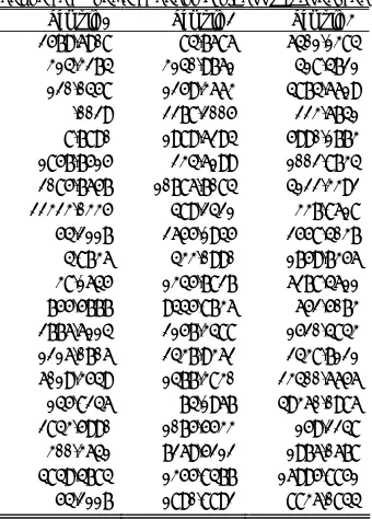
314.3274 3140.9761 418.4721 120.0458 1259.3663 4874.6619 .0029 2278.2005 223.6741 8.7890 1989.6294 5990.1773 1857.7515 234.6199 1002.8734 2085.7657 10786.7084 4122.3392 22323.0335 489.2421 337.8618

54.2117 2655.1945 2558.4037 4.8736 433.0990 1759.7356 38.1645 1345.7827 6278.4611 755.5777 9445.8736 652.5073 2776.6114 2157.3488 1520.4843 1216.0706 2437.9362 2438.7121 6019.3549 1477.3830 23400.6656

145.8246 74.1967 49360.0986

2843.5990 1075.5533 159.2248 300.3641 7269.5212 1976.0678 4849.4784 1355.8477 16995.8851 54.2117 1890.8892 8836.0844

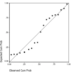
The Normal P-P plot for each sample is presented in Fig. 1-3. The results show that each sample of data is non-normal.

Observed Cum Prob

1.00 .75 .50 .25 0.00

Ex

pe

cte

d Cum P

rob

1.00

.75

.50

.25

0.00

Fig. 1Normal P-P plot of data from Sample 1

Observed Cum Prob

1.00 .75 .50 .25 0.00

Ex

pe

cted

Cum P

rob

1.00

.75

.50

.25

0.00

Observed Cum Prob

1.00 .75 .50 .25 0.00

Ex

pe

cted

Cum P

rob

1.00

.75

.50

.25

0.00

The Weibull P-P plot for each sample is presented in Fig. 4-6. The results show that each sample of data is Weibull.

Observed Cum Prob

1.00 .75 .50 .25 0.00

Ex

pe

cte

d Cum P

rob

1.00

.75

.50

.25

0.00

Fig. 4 Weibull P-P plot of data from Sample 1

Observed Cum Prob

1.00 .75 .50 .25 0.00

Ex

pe

cted

Cum P

rob

1.00

.75

.50

.25

0.00

Fig. 5 Weibull P-P plot of data from Sample 2

Observed Cum Prob

1.00 .75 .50 .25 0.00

Ex

pe

cted

Cum P

rob

1.00

.75

.50

.25

0.00

Fig. 6Weibull P-P plot of data from Sample 3

[image:3.595.84.254.169.406.2] [image:3.595.367.491.274.394.2] [image:3.595.373.494.427.544.2] [image:3.595.113.237.456.577.2] [image:3.595.373.494.577.697.2] [image:3.595.108.231.608.728.2]

(4)

Hence, the transformation for this Weibull data set is

-0.069318

0.01 1

-0.069318

⎡ + ⎤ −

⎣ ⎦

= ij i

ij

X c

Y . (10)

The transformed data are shown in Table II.

TABLEII THE TRANSFORMED DATA

Sample 1

Sample Sample 2 3

6.1053 4.4056 6.6085 5.0962 6.1899 5.4308 4.8015 5.6805 6.4717 4.5101 6.0118 5.2794 4.5366 5.9362 6.5751 5.9318 4.7986 5.7347 5.9928 6.8526 6.3880 7.2250 5.1631 5.3728 4.6584 6.0969 6.1540 4.5250 5.0994 5.9781 4.6180 5.7176 6.5988 5.4758 6.7834 5.5723 6.1444 5.9814 5.9120 5.7119 6.0495 6.1310 6.5546 5.7697 7.2539 4.8497 4.3662 7.6104 6.1571 5.5924 5.2194 5.0791 6.6452 6.0316 6.4406 5.7217 7.0971 4.6584 5.9078 6.7707

In general, the usual basic assumptions, normality in each group of data and homogeneity of variances, should be validated before ANOVA is applied and so these assumptions should be tested. The normal P-P plot for each sample of transformed data is presented in Fig 7-9. The results show that each sample of transformed data is normal.

Observed Cum Prob

1.00 .75 .50 .25 0.00

Ex

pe

cted

Cum P

rob

1.00

.75

.50

.25

0.00

Fig. 7Normal P-P plot of transformed data from Sample 1

Observed Cum Prob

1.00 .75 .50 .25 0.00

Ex

pe

cted

Cum P

rob

1.00

.75

.50

.25

0.00

Observed Cum Prob

1.00 .75 .50 .25 0.00

Ex

pe

cted

Cum P

rob

1.00

.75

.50

.25

0.00

The Levene statistic * L

F of transformed data is 1.571. For significance level

α =

0.05

, F0.05,2,57=3.15. Since

* L

F =1.571 < 3.15, They have a constant variance. The ANOVA assumptions of the transformed data are checked and are valid. Subsequently the transformed data are used to test the equality of the population means using ANOVA. The results are shown in Table III.

TABLEIII

ANOVATABLE FOR H0:μ1=μ2=μ3

Source of Variation df Sum of Squares Mean Square F-ratio

Between treatment 2 5.830 2.915 5.418

Within treatment 57 30.684 0.538

Total 59 36.514

The F test statistic, F 5.418= , and F0.05,2,57 =3.15. Since F 5.418= > 3.15, there is a significant difference in at least one pair among the three population means.

V. ANUMERICAL STUDY

In order to attain the most effective use of the proposed transformation, we set the values of parameters and the significant value as follows:

1) k= number of the populations = 3,

2) n = sample size from the i th Weibull population i =10, 20, 30, 50,

[image:4.595.373.493.86.207.2] [image:4.595.81.254.161.410.2] [image:4.595.115.236.502.625.2] [image:4.595.304.550.515.584.2]

(5)

is between 1000 and 4000,

4) αi= shape parameter of the i th Weibull population is between 1 and 1.5,

5) Significant level = 0.05.

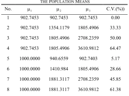
The Weibull populations of size Ni = 4,000 (i 1, 2,3)= are generated for different values of parameters α βi, i shown in Table IV.

TABLEIV

THE VALUES OF PARAMETERS α_iANDβ_i

No. Values of Parametersαiandβ_i

1 α =1 1.5,α =2 1.5,α =3 1.5,β =1 1000,β =2 1000,β =3 1000

2

1 1.5, 2 1.5, 3 1.5, 1 1000, 2 1500, 3 2000

α = α = α = β = β = β =

3 α =1 1.5,α =2 1.5,α =3 1.5,β =1 1000,β =2 2000,β =3 3000

4 α =1 1.5,α =2 1.5,α =3 1.5,β =1 1000,β =2 2000,β =3 4000

5 α =1 1.0,α =2 1.2,α =3 1.5,β =1 1000,β =2 1000,β =3 1000

6 α =1 1.0,α =2 1.2,α =3 1.5,β =1 1000,β =2 1500,β =3 2000

7 α =1 1.0,α =2 1.2,α =3 1.5,β =1 1000,β =2 2000,β =3 3000

8 α =1 1.0,α =2 1.2,α =3 1.5,β =1 1000,β =2 2000,β =3 4000

From aWeibull( , )α βi i , 1,000 random samples, each of size i

n , are drawn. Then we transform each set of the sample data to normality by the proposed transformation. The differences among the population means are measured by the coefficient of variation (C.V.) shown in Table V.

TABLEV

THE COEFFICIENT OF VARIATION AMONG THE POPULATION MEANS

No. μ1 μ2 μ3 C.V.(%))

1 902.7453 902.7453 902.7453 0.00

2 902.7453 1354.1179 1805.4906 33.33

3 902.7453 1805.4906 2708.2359 50.00 4 902.7453 1805.4906 3610.9812 64.47 5 1000.0000 940.6559 902.7403 5.17 6 1000.0000 1410.984 1805.4906 28.66 7 1000.0000 1881.3117 2708.2359 45.85 8 1000.0000 1881.3117 3610.9812 61.38

A. Check Validity of Assumption

The results of the goodness- of-fit tests and the tests of homogeneity of variances with 1,000 replicated samples of various sizes are shown in Table VI to Table IX.

TABLEVI

AVERAGES OF THE P-VALUES FOR K-STEST OF NORMALITY, AND OF THE P-VALUES FOR THE LEVENE TEST USING DATA TRANSFORMED

BY THE ALTERNATIVE TRANSFORMATION WITH ni=10

TABLEVII

BY THE ALTERNATIVE TRANSFORMATION WITH ni=30

TABLEVIII

BY THE ALTERNATIVE TRANSFORMATION WITH ni=50 No. Averages of the p-Values for _{K-S Test}

of Transformed Data

Averages of the p-Values

for the Levene Test

1 0.815935 0.836797 0.832448 0.512381

2 _{0.833253 0.830454 0.830982 0.500592}

3 0.807439 0.812730 0.832753 0.505986

4 0.818064 0.809636 0.821178 0.517538

5 0.837132 0.840045 0.822093 0.464288

6 0.833911 0.832420 0.823324 0.487294

7 0.842745 0.833669 0.803619 0.571945

8 0.826983 0.828171 0.815086 0.584423

No. Averages of the p-Values for _{K-S Test} of Transformed Data

for the Levene Test

1 0.701827 0.702871 0.767305 0.496945

2 _{0.681334 0.642862 0.655129 0.374862}

3 0.633572 0.611771 0.571767 0.328161

4 0.525433 0.523030 0.512390 0.245224

5 0.761650 0.753825 0.638876 0.289726

6 0.744558 0.772147 0.629379 0.408814

7 0.745982 0.684544 0.566321 0.566636

8 0.740399 0.700717 0.592849 0.518817

No. Averages of the p-Values for _{K-S Test} of Transformed Data

for the Levene Test

1 0.596132 0.541692 0.633408 0.511615

2 _{0.573105 0.458770 0.504397 0.282900}

3 0.487750 0.422268 0.346918 0.211742

4 0.442299 0.331097 0.366252 0.196322

5 0.652811 0.661944 0.432919 0.203807

6 0.672854 0.686797 0.413016 0.371272

7 0.648873 0.521054 0.346788 0.524520

[image:5.595.65.271.469.623.2]

(6)

TABLEIX

AVERAGES OF THE P-VALUES FOR K-STEST OF NORMALITY, AND OF THE P-VALUES FOR THE LEVENE TEST USING DATA TRANSFORMED BY THE ALTERNATIVE TRANSFORMATION WITH n1=10,n2=20,n3=30

We have seen that, all sets of the Weibull data transformed by the alternative transformation can be checked by the K-S test and for homogeneity of variances by the Levene test. Furthermore, they always meet all the required assumptions for ANOVA.

B. Powers of the ANOVA Test

We transform each set of the sample data to normality and homogeneity of variances by proposed alternative

transformation. Then the transformed data sets are used to test the equality of the population means by ANOVA. The power of the F-test as obtained from ANOVA given by Patnaik [10] is

1

( ,..., ) ( )

∞

′ ′ =

_∫

k F

p F dF

α

β μ μ

2 2 1

1 ( ) ₂

2

2 1 0

( )

1 2

.

1 1

! ( 1) , ( )

2 2

= − − ∞

= =

∑ ⎛ − ⎞

⎜ ⎟

⎝ ⎠

=

⎛ _{− +} ₋ ⎞

⎜ ⎟

⎝ ⎠

∑

k i i i

n t

k

i i

i t

n e

t B k t n k

μ μ

σ μ μ

σ

1_{( 1)} 1_{( 1)}

1

2 ( 1) 1 2

2

( 1) ₁ ( 1)

( ) ( )

− + − − −

∞_⎛ ₋ _⎞ _{− − +}_⎛ ₋ _⎞

′ + ′ ′

⎜ ₋ ⎟ ⎜ ₋ ⎟

⎝ ⎠ ⎝ ⎠

∫

k t k t n t

F

k k

F F dF

n k n k

α

(11) where

1

=

∑

ni

i ij

j i

y n

μ ,

1 1

1

= =

=

∑∑

k ni

ij

i j

y n

μ , and 2 2

1 1

1

( )

= =

=

∑∑

k ni −

ij

i j

y n

σ μ .

The results of the power of the ANOVA tests with 1,000

replicated samples of various sizes are shown in Table X.

TABLEX

POWERS OF THE ANOVATESTS OF EQUALITY OF MEANS

USING TRANSFORMED DATA

Power of the ANOVA Test

No. 1 2

3 10 = = =

n n

n

1 2

3 30 = = =

n n

n

1 2

3 50 = = =

n n

n

1 2

3

10,

20, 30

= =

=

n n

n

1 0.047946 0.051030 0.053016 0.048728

2 _{0.286518 0.669822 0.816144 0.319087}

3 0.584186 0.917247 0.979087 0.670549 4 0.769037 0.983201 0.999780 0.866752 5 0.063552 0.067198 0.077095 0.070527 6 0.470168 0.811293 0.918057 0.625139 7 0.626333 0.899473 0.969276 0.710698 8 0.816969 0.981594 0.998056 0.879196

We see that the power of the ANOVA test increases as n_i

increases. Furthermore, when the differences among the population means are larger, higher powers of the tests are obtained.

VI. CONCLUSION

The alternative transformation as proposed in this paper is applied to transform Weibull data to Normal data with constant variance. The numerical results indicated that the Weibull data sets transformed by the alternative

transformation always meet the assumptions required for the application of ANOVA. The power of the test depends on the sample sizes, and also on the shape and scale parameters of the populations.

REFERENCES

[1] W. Tukey, “On the comparative anatomy of transformations,” Annals of Mathematical Statistics, vol. 23, 1957, pp.525-540.

[2] D. C. Montgomery, Design and Analysis of Experiments, 5thed.New York: Wiley, 2001, pp. 590.

[3] G. E. P. Box and D. R. Cox, “An analysis of transformations (with discussion),” Journal of the Royal Statistical Society, Ser.B. vol. 26, 1964, pp.211-252.

[4] J. Schlesselman, “Power Families: A Note on the Box and Cox Transformation,” Journal of the Royal Statistical Society, Ser. B. vol. 33, 1971, pp.307-311.

[5] B. F. J. Manly, “Exponential Data Transformations,” Statistician. vol. 25, 1976, pp.37-42.

[6] J. A. John and N. R. Draper, “An alternative family of transformations,” Applied Statistics, vol. 29(2), 1980, pp.190-197.

[7] K. A. Doksum, and C. Wong, “Statistical tests based on transformed data,” Journal of the American Statistical Association, vol. 78, 1983, pp. 411-417.

[8] N. L. Johnson, and S. Kotz, Continuous Univariate Distributions. New York: Wiley, 1970.

[9] A. Chaudhuri, and N. K. Chandra, “A Test for Weibull Populations,” Statistics & Probabilty Letters, vol. 7, 1989, pp. 377-380.

[10] P. B. Patnaik, “The non-central