Abstract— This work presents a differential evolution algorithm for solving a single-item resource-constrained aggregate production planning (APP) problem. Due to its NP-hardness, we have developed a Differential Evolution (DE) for solving the above model with a real representation of chromosomes, adapting DE with the integer nature of the problem. Experiments were carried out to compare results from the differential evolution algorithm and local optimum solutions obtained by optimization software.
Keywords— Aggregate production planning, Differential evolution, Optimization.
I. INTRODUCTION
Aggregate production planning belongs to a class of production planning problems in which there is a single production variable representing the total production of all products [1]. The term Aggregate indicate that all production must be treated as one and there must be some units for measuring the aggregate output that is called "aggregate unit of production" such as tons for a steel mill, machine-hours for a job shop or man-hours for a maintenance department.
APP deals with matching capacity to demand fluctuation, varying customer orders over the medium term, often from 3 to 18 months in advance [2]. The main goal of APP is setting overall production levels for each product group by managing the hiring, layoffs, backorders, overtimes, subcontracting and inventory level to meet uncertain demand in the near future.
APP has attracted considerable attention from both practitioners and academia [3]. In the field of planning, it falls between the broad decisions of long-range planning and the highly specific and detailed short-range planning decisions. APP is one of the most important functions in
Manuscript received December 29, 2007 and revised on January 16,2008.
Maryam earned a bachelor's degree in industrial engineering from Iran University of Science and Technology, Tehran-IRAN. She is now working on her thesis in order to earn a master's degree in industrial engineering. Her research has focused on evolutionary Algorithms and production management problems (phone: 00982144332971; e-mail: Maryam_Mhj@ yahoo.com).
Dr. Farid Khoshalhan is an assistant professor in Industrial Engineering and Information Technology at Faculty of Industrial Engineering, K.N.Toosi University of Technology, Tehran-IRAN. His research and client work has focused on inventory and production management, evolutionary algorithms, performance and productivity management and e-commerce. Dr. Khoshalhan earned a bachelor's degree in industrial technology from Iran University of Science andTechnology, a master's and PhD in industrial engineering from Tarbiat Modarres University in IRAN.
Tell:+9821-88678580 Email: ([email protected])
production and operations management. Other forms of family disaggregation planning involve a master production schedule, capacity requirements planning, material requirements planning, which all depend on APP in a hierarchical way [2].
Since the HMMS rule was proposed in 1955, researchers have developed numerous models to help to solve the APP problem [4].
All traditional models of APP problems may be classified into six categories [5] — (1) linear programming (LP) [6], (2) linear decision rule (LDR) [4], (3) transportation method [7], (4) management coefficient approach [8], (5) search decision rule (SDR) [9], and (6) simulation [10].
Also, some of heuristic APP strategies to satisfy demand are discussed in details in the literature [11]. Some of these yield the optimal solution; whiles others give only acceptable ones. Solving APP model is affected by problem size and type of cost functions (linear, non-linear or both of them). Studies show that the consideration of the all realistic parameters in an APP model makes the model difficult and non-optimally solvable. Therefore, it is necessary for a trade-off between the selection of a non-exact model with an optimal solution and an exact model with a near-optimal solution [1]. Nowadays metaheuristic methods are widely used to obtain near optimal solution for NP-hard problems such as generalized APP and the like.
Among the numerous method capable of developing mathematical optimization models include APP problems, a literature survey reveals that linear programming is conventionally used technique [12].
Some literatures considers solving different kind of APP models using genetic algorithms that shows robust to obtain near optimal solution in more reasonable time in comparison with traditional techniques such as branch and bound.
Additional references on the use of FLP to solve APP problems include [13], [14], [15], [16], and [17].
The rest of paper is organized as follows. Section II describes the APP problem and model. Section III introduces the DE and considers its adaptation to solve the model. Some numerical results are included in section IV and concluding remarks are made in section V.
II. PROBLEM FORMULATION
The single-item resource constrained problem is a nonlinear model of APP considering four main costs as production, adjusting work forces, inventory carrying and shortage ones. In this model, all resources are assumed to be finite and backorder is allowed to a level determined by customer but the ending shortage is not permitted. Available time for manpower in regular time and overtime, subcontracting level, storage area and adjusting work force level depends on the decision maker.
Application of Differential Evolution for a Single-Item
Resource-Constrained Aggregate Production Planning Problem
The demand rate assumed to be deterministic and dynamic under a multi period horizon planning and the initial value for each parameter is known before. The model was linearized to a mixed integer one [1]. The Proposed model was modified and described below.
A. Notation
T=number of periods in horizon planning. Dt=forecasted demand in period t. I0=beginning inventory.
W0=initial workforce level.
Imax=maximum inventory available in period t (units). Bmax=maximum backorder (shortage) available in period t (units).
Hmax=maximum allowable hiring at each period. Fmax=maximum allowable firing at each period.
Rmax=maximum production volume in regular time at each period (units).
Rmax=maximum production volume in overtime at each period (units).
Smax= maximum production volume in subcontracted available at each period (units).
rt=regular time production cost per unit in period t ($/unit).
ot= overtime production cost per unit in period t ($/unit). st= subcontracting cost per unit in period t ($/unit). ht=hiring cost per one worker in period ($/man). ft= firing cost per one worker in period ($/man). h+
t=inventory carrying cost per unit in period ($/man). h
-t=backorder cost per unit in period ($/man). k=number of workers required per unit product Decision Variables
Pt=total aggregate production in period t.
Rt=regular time production volume in period t (units). Ot=overtime time production volume in period t (units). St=subcontracting production volume in period t (units). Ht=workers hires in period t.
Ft=workers fires in period t.
It=inventory/backorder level in period t (negative inventory ≡ shortage).
B. Mathematical Formulation
By defining the above notation, the mathematical model of APP can be presented as follows.
∑
, 0 , 0 (1)
. . (2)
(3)
(4)
1 (5)
(6)
(7)
(8)
max , 0 (9)
max , 0 (10)
(11)
(12)
max , 0 0 (13)
, , , , , (14)
The nonlinear objective function (1) is equal to the total cost of production, adjusting workforce, inventory carrying, and shortage in planning horizon. Equation (2) indicates the balance inventory constraint between periods. Equation (3) determines the total production level at each period. Equations (4) and (5) calculates the number of workers hired/fired at each period with respect to the total regular and overtime production level. Inequalities (6) to (8) correspond to the maximum allowable volume of production in regular time, overtime and subcontracting at each period respectively. Inequalities (9) and (10) correspond to maximum allowable level of inventory and backorder (shortage) at each period respectively. Likewise, inequalities (11) and (12) correspond to maximum allowable level of hiring and firing at each period respectively. Finally equation (13) indicates the lack of shortage at the end of horizon planning. The mentioned model includes 10T constraints and 7T integer variables, where T is the number of periods in horizon planning.
III. DIFFERENTIAL EVOLUTION
In 1997, a new Evolutionary algorithm known as Differential Evolution (DE) was successfully applied by [18] to the optimization of some well-known and non-convex functions. This technique combines simple arithmetic operators with the classical events of crossover, mutation and selection to evolve from a randomly generated starting population to a final solution [19].
DE can be categorized to the class of floating point encoded, evolutionary optimization algorithms. Currently, there are several variants of DE and the most popular one is DE/rand/1/bin [20]. The Different DE schemes are discussed more detailed in [20],[21].
DE can be categorized to the class of floating point encoded, evolutionary optimization algorithms. Currently, there are several variants of DE and the most popular one is DE/rand/1/bin [20]. The different variants are classified using the following notation:
DE/X/Y/Z where:
X indicates method for selecting the parent chromosome that will form the base of the mutated vector. Thus, DE/best/1/bin selects the best member of the population to form the base of the mutated chromosome.
Y indicates the number of difference vectors used to perturb the base chromosome.
Z indicates the crossover mechanism used to create the child population. The bin acronym indicates that crossover is controlled by a series of independent binomial experiments [19].
Generally, the function to be optimized, f(X), is the form of f(X): RD→R. The optimization target is to minimize the value of this objective function f(X),
Min (f(X)),
By optimizing the value of its parameters X={x1, x2,…, xD}, where X denotes a vector composed of D objective function parameters. Usually, the parameters of the objective function are also subject to lower and upper boundary constraints, xL and xU respectively,
A. Chromosome Representation
The first step of any kind of evolutionary algorithms is to design and represent a proper chromosome for the solution structure coding. This structure must be compatible with the model's decision variables and constraints. According to the mentioned model, each solution is represented by a chromosome formed as an integer vector with T genes as shown in Figure 1, where T is the number of periods [1]. The value of tthgene, i.e, P
t, indicates the total production in period t that is bounded in interval [0, Rmax, Omax, Smax].
B. Initialization
As with all evolutionary optimization algorithms, DE works with a population of solutions, not with a single solution for the optimization problem. Population P of generation G contains NP solution vectors called individuals of the population and each vector represents potential solution for the optimization problem [20].
The initial population is generated randomly in the way that boundary constraints are satisfied, the more divers initial population increase the chance of reach the optimal solution. In this case a natural way to initialize the population P(0) (initial population) is to seed it with random values within the given boundary constraints.
C. Mutation
The self-referential population recombination scheme of DE is different from other evolutionary algorithms. For mutating each population P(G), first a temporary or trial population is generated according to selected strategy. In this study, we discussed DE/best/1/bin, so the trial vector, vj,i(G) is generated as follows:
, , , , (15)
Where 1, , 1, , 1, 2
1, , randomly selected, except: 1 2 ,
0,1 1 and 0,1 , 0,1 .
Two randomly chosen index, r1,r2, refer to two randomly chosen vectors of population, and best is index of the best vector in the population [20].
D. Crossover
The crossover process is a series of independent binomial trials. It determines if the vector parameter value for the child chromosomes will come from the mutated vector or from the target vector in the corresponding position in the parent population. If a random variable was less than or equal to CR, then the vector parameter value is taken from the mutated vector. Otherwise, the vector parameter value is taken from the target vector in the corresponding position in the parent population [19].
Trial Vector U1 U2 U3 U4 U5
ra
nd<CR
ra
nd<CR
ra
nd<CR
Target Vector P1 P2 P3 P4 P5
ra
nd>CR
ra
nd>CR
[image:3.595.341.514.58.214.2]Offspring U1 P2 U3 P4 U5 Fig 2. Crossover operator
Binomial crossover products a single offspring by probabilistic combining target vector and trial vector as shown in Figure 3.
,
, , 0,1 ,
,
(16)
The index k refers to a randomly chosen vector parameter and it is used to ensure that at least one vector parameter value of each child is differs from its counterpart in the parent population.
E. Selection
The selection scheme of DE also differs from the other evolutionary algorithms. Vectors in the child population are compared for fitness to the target vectors and vector with better fitness function survives in to the next generation.
F. Handling Constraints
1) Boundary Constraints
It is important to notice that the mutation scheme of DE is able to extend the search outside the defined boundaries, so it is essential to ensure that parameter values lie inside their allowed range. A simple way to guarantee the feasibility of parameters is to replace parameter values that violated the boundary constraints with random value generated within the feasible range, in the way that violated vector parameter greater that upper bound is replaced with a random value between target vector parameter and upper bound and if vector parameter value is less than lower bound, it will be replaced with random value between lower bound and target vector parameter. Since in our problem, lower and upper limit for all parameter values are the same, [0, Rmax, Omax, Smax], so the below formula is used for this purpose.
,
0,1 , , 0,
, 0,1 U , , , U,
, ,
(17)
Where R O S , 1, , 1, .
In fact this operation is a kind of migration, not only brings the infeasible mutated vector parameter into feasible region,
1 2 3 T
[image:3.595.90.232.180.220.2]P1 P2 P3 PT
but also proper diversity is obtained in order to DE stagnation.
2) Integer Variables
In the canonical form, the differential evolution algorithm is only capable of handling continuous variables. Some studies discuss how to modify DE for mixed integer variable optimization, the suggested method uses only a copy of vector parameters and converts it to integer values then evaluates the fitness function, even though DE still work with continuous floating point values [21].
3) Functional Constraints
An excellent study on comparing evolutionary algorithms for constrained optimization problems [22], the methods are grouped into the following four categories:
• Methods based on preserving feasibility of solution. • Methods based on penalty functions.
• Methods based on a search for feasible solutions. • Other hybrid methods.
Among the evolutionary algorithms the methods based on penalty function have been proven to be the most popular [23]. In this study we use penalty function to handle these kinds of constraints.
According to the chromosome representation, other decision variables must be updated with respect to the current solution and the model constraints by equations (18) to (23).
min , (18)
min , max , 0 (19)
min , max , 0 (20)
(21)
max , 0 (22)
max , 0 (23)
Where P0=W0/k and I0 are known as priori. Equation (13) indicates that total production and initial inventory must not less than total demand over horizon planning, ∑ ∑ . If one of the constraints (9) to (13) are violated by on hand solution, then the degree of violation is added to the objective function by the penalty coefficient λ, that is a large positive number. Equation (24) indicates the fitness function that chromosomes are evaluated by the following equation. ∑ , 0 , 0 ∑ max 0, max 0, max 0, max (24)
IV. EXPERIMENTAL RESULTS
A. Parameter Tuning
The values of NP, CR and F are fixed empirically following certain heuristics [18].F is usually between 0.5 and 1.0 and CR usually should be 0.3, 0.7, 0.9 or 1.0 to start with.NP should be of the order of 10 * D and should be increased in case of miss-convergence. If NP is increased then usually F has to be decreased [19]. In this study, twenty trials were carried out consisting of four mentioned levels of CR, five levels of F (0.3, 0.5, 0.7, 0.9 and 1) and three levels of NP (3*D,8*D and 10*D). The best values obtained from
combining these parameters during experimentation are F = 0.5, and CR = 0.3 and the population size was set to eight times of period number, Another parameter is penalty coefficient in equation (24) that is set to 10000 in order to reduce the infeasibility of the problem. Previous studies showed that DE/rand/1/bin is the most popular among ten strategies of DE, so we examined here two DE strategies: DE/rand/1/bin and DE/best/1/bin. We also we experimented DE local search [24] which assumes that the target vector is the main parent in the mutation scheme. The results for T= 70 are shown in table I.
Table I. Comparing the results of DE strategies using 70 periods problem Strategy DE/rand/1/bin DE/best/1/bin* DE local search Fitness value 2112315 2109126 2230111
*Best Strategy
B. Numerical example
In this section, several instances are solved by coded DE in MATLAB and run it on a PC with Pentium, 3 GHz processor and 1 GB of RAM. The results are compared with local optimum obtained by Lingo software package, using branch & bound method. Table II shows one sample of the generated data for this problem, the intervals are adapted from the presented data in the literature [1].
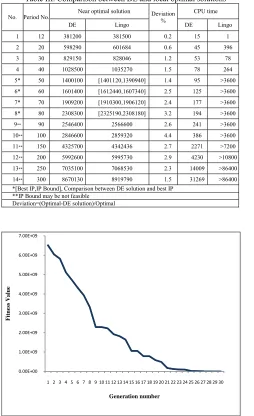
Table 3 illustrated the comparison between solutions obtained by DE and local optimal solutions, the results are compared with respect to the mean objective value, and the mean CPU time to 15 instances according to the table III.
As shown in table 3, increasing period numbers has a considerable effect on the computational correspond CPU time in both DE and local optimal solution. The results indicate that DE could find better solutions in comparison with local optimums and could find the near optimal solutions in a reasonable time. This is considerable when period number is increased to over than 50.
[image:4.595.318.553.511.625.2]In fact DE has a strong capability to reduce the infeasibility of the problem, figure 3 shows DE trend toward a near optimal solution in less than 30 generation and figure 4 shows a typical convergence of DE to a feasible solution during about 27 generations at T=40 (period number=40).
Table II. Intervals to random generation of instance
Parameter Interval Parameter Value
dt U(Pmax-δ,Pmax-δ) I0 2000
rt U(10,20) W0 480
ot U(20,30) Imax 2000
st U(30,40) Bmax 1000
ht U(100,150) Hmax 200
ft U(200,250) Fmax 100
ht+ U(1,10) Rmax 2400
ht- U(10,20) Omax 400
Smax 200
Fig 3. A typical convergence of DE to near optimal solution
Fig 4. Decreasing trend of penalty using DE
V. CONCLUSION
In this work, an aggregate production planning model was considered with the most realistic costs and parameters. To
solve such a NP-Hard problem, a differential evolution algorithm was proposed and made compatible with integer nature of the problem. The numerical results indicates that DE has a strong capability in reducing the infeasibility of the problem, in fact the penalty function and migration was so well designed to bring the problem into the feasible space in few generations. Since the migration operator provides more diversity in generations, it prevents DE from stagnation. The described method is relatively simple, easy to implement and easy to use. It is, however, capable of optimizing all integers, discrete and continuous variables and capable of handling non-linear objective functions with multiple non-trivial constraints. The proposed DE can be applied in other industrial engineering problems like lot sizing problems and inventory models, and also other evolutionary algorithm can be applied for the considered model in the future research.
ACKNOWLEDGMENT
Kenneth Price made the concept of differential evolution clear and his guides in order to handle different kinds of constraints are appreciable.
REFERENCES
[1] R. Tavakkoli-Moghaddam, N. Safaei, “ An evolutionary algorithm for a single-item resource-constrained aggregate production planning,” in
IEEE Congress on Evolutionary Computation, 2006, pp. 2851-2858.
[2] R.C. Wang, T. F. Liang, “Application of fuzzy multi-objective linear programming to aggregate production planning,” Computer and
industrial engineering, vol. 46, 2004, pp. 17-41.
[3] Y. Shi, C. Haase, “Optimal trade-offs of aggregate production planning with multi-objective and multi-capacity- demand levels,” International
Journal of Operations and Quantitative Management, 1996, pp
127-143.
[4] C. Holt, C. Modigliani, F., Simon, H. A. “Linear decision rule for production and employment scheduling,” Management Science, vol. 2, 1995, pp 1–30.
[5] G. Saad, “An Overview of Production Planning Model: Structure Classification and Empirical Assessment,” International Journal of
Production Research, 1982, pp 105-114.
[6] A. Charnes, W.W. Cooper, “Management models and industrial
applications of linear programming,” New York: Wiley, 1961.
[7] Bowman, E.H., “Production Scheduling by the Transportation Method of Linear Programming,” Operations Research, vol. 2, 1956, pp.
100-103.
[8] E.H. Bowman, “Consistency and Optimality in Managerial Decision Making,” Management Science, vol. 9, 1963, pp. 310-321.
[9] Taubert, W.H., “A Search Decision Rule for the Aggregate Scheduling Problem,” Management Science, vol. 14, 1968, pp. 343-359.
[10]C. H. Jones, “Parametric production planning,” Management Science, vol. 13, 1967, pp. 843–866.
[11]Fogarty, Blackstone & Hoffmann, Production and inventory
management, 2th- edition, south western publishing, 1991, ch. 1.
[12]R. C. Wang, H.H. Fang, “Aggregate Production Planning with Multiple Objectives in a Fuzzy Environment,” European journal of
operational research, vol. 133, 2001, pp. 521-536.
[13]Y. Y. Lee, “Fuzzy Set Theory Approach to Aggregate Production planning and inventory control.” PhD Dissertation. Department of I.E., Kansas State University, 1990.
[14]A. S. Masud, C. L. Hwang, “An aggregate production planning model and application of three multiple objective decision methods,”
International Journal of Production Research, vol. 18, 1980, pp.
741–752.
[15]D. B. Rinks, “The performance of fuzzy algorithm models for aggregate planning and differing cost structure,” In M. M. Gupta, & E. Table III. Comparison between DE and local optimal solutions
No. Period No. Near optimal solution Deviation % CPU time DE Lingo DE Lingo
1 12 381200 381500 0.2 15 1
2 20 598290 601684 0.6 45 396
3 30 829150 828046 1.2 53 78
4 40 1028500 1035270 1.5 78 264
5* 50 1400100 [1401120,1390940] 1.4 95 >3600 6* 60 1601400 [1612440,1607340] 2.5 125 >3600
7* 70 1909200 [1910300,1906120] 2.4 177 >3600 8* 80 2308300 [2325190,2308180] 3.2 194 >3600
9** 90 2546400 2566600 2.6 241 >3600 10** 100 2846600 2859320 4.4 386 >3600
11** 150 4325700 4342436 2.7 2271 >7200 12** 200 5992600 5995730 2.9 4230 >10800
13** 250 7035100 7068530 2.3 14009 >86400 14** 300 8670130 8919790 1.5 31269 >86400 *[Best IP,IP Bound], Comparison between DE solution and best IP
**IP Bound may be not feasible Deviation=(Optimal-DE solution)/Optimal
0.00E+00 1.00E+09 2.00E+09 3.00E+09 4.00E+09 5.00E+09 6.00E+09 7.00E+09
1 2 3 4 5 6 7 8 9 10 11 12 13 14 15 16 17 18 19 20 21 22 23 24 25 26 27 28 29 30
F
itness Value
Generation number
0.00E+00 5.00E+04 1.00E+05 1.50E+05 2.00E+05 2.50E+05 3.00E+05
1 2 3 4 5 6 7 8 9 10 11 12 13 14 15 16 17 18 19 20 21 22 23 24 25 26 27
Infe
asibilit
y
[image:5.595.47.288.518.704.2]Sachez (Eds.), Approximate reasoning in decision analysis,
Amsterdam: North-Holland, pp. 267–278.
[16]D. Wang, R. Fung, “Fuzzy formulation for multi-product aggregate production planning,” Production Planning and Control, vol. 11,
2000, pp. 670–676.
[17]R. C. Wang, H.H. Fang, “Aggregate production planning with multiple objective in a fuzzy environment,” European journal of operational
research, vol. 133, 2001, pp. 521-536.
[18]R. Storn, K. V. Price, “Differential Evolution - A Simple and Efficient Heuristic for Global Optimization over Continuous Spaces,” Journal
of Global Optimization, 1997, pp. 341-359.
[19]P.Bergeya, C. Ragsdaleb, “Modified Differential Evolution: a Greedy random Strategy for Genetic Recombination,” The International
Journal of Management Science, vol. 33, 2005, pp. 255-265.(VOL)
[20]O. Godfrey, D. Donald, “Scheduling Flow Shops Using Differential Evolution Algorithm,” European Journal of Operational Research,
vol. 171, 2006, pp. 674-692.
[21]J. Lampinen, I. Zelinka, “Mechanical Engineering Design Optimization by Differential Evolution,” In: Corne, D., Dorigo, M., Glover (Eds.), New Ideas in Optimization. McGraw Hill, International
(UK), 1999, pp. 127-146.
[22]Z. Michalewics, M. Schoenauer, “Evolutionary algorithms for constraint parameter optimization problems,” Evolutionary
Computation, vol. 4(1), 1996, pp. 1–32.
[23]H. Sarimveis, A. Nikolakopoulos, “A line up evolutionary algorithm for solving nonlinear constrained optimization problems,” Computers
and operations research, vol. 32, 2005, pp. 1499-1514.
[24]K. V. Price, J. Rönkkönen, “Comparing the Uni-Modal Scaling Performance of Global and Local Selection in a Mutation-Only Differential Evolution Algorithm,” Proceedings of 2006 IEEE World
Congress on Computational Intelligence (CEC06), 2006, pp.