A Comparison of Algorithms for Maximum Entropy Parameter Estimation

(1)

A comparison of algorithms for maximum entropy parameter estimation

Robert Malouf

Alfa-Informatica Rijksuniversiteit Groningen

Postbus 716 9700AS Groningen

Abstract

Conditional maximum entropy (ME) models pro-vide a general purpose machine learning technique which has been successfully applied to fields as diverse as computer vision and econometrics, and which is used for a wide variety of classification problems in natural language processing. However, the flexibility of ME models is not without cost. While parameter estimation for ME models is con-ceptually straightforward, in practice ME models for typical natural language tasks are very large, and may well contain many thousands of free parame-ters. In this paper, we consider a number of algo-rithms for estimating the parameters of ME mod-els, including iterative scaling, gradient ascent, con-jugate gradient, and variable metric methods. Sur-prisingly, the standardly used iterative scaling algo-rithms perform quite poorly in comparison to the others, and for all of the test problems, a limited-memory variable metric algorithm outperformed the other choices.

1 Introduction

Maximum entropy (ME) models, variously known as log-linear, Gibbs, exponential, and multinomial logit models, provide a general purpose machine learning technique for classification and prediction which has been successfully applied to fields as di-verse as computer vision and econometrics. In natu-ral language processing, recent years have seen ME techniques used for sentence boundary detection, part of speech tagging, parse selection and ambigu-ity resolution, and stochastic attribute-value gram-mars, to name just a few applications (Abney, 1997; Berger et al., 1996; Ratnaparkhi, 1998; Johnson et al., 1999).

A leading advantage of ME models is their flex-ibility: they allow stochastic rule systems to be augmented with additional syntactic, semantic, and pragmatic features. However, the richness of the

representations is not without cost. Even mod-est ME models can require considerable computa-tional resources and very large quantities of anno-tated training data in order to accurately estimate the model’s parameters. While parameter estima-tion for ME models is conceptually straightforward, in practice ME models for typical natural language tasks are usually quite large, and frequently contain hundreds of thousands of free parameters. Estima-tion of such large models is not only expensive, but also, due to sparsely distributed features, sensitive to round-off errors. Thus, highly efficient, accurate, scalable methods are required for estimating the pa-rameters of practical models.

In this paper, we consider a number of algorithms for estimating the parameters of ME models, in-cluding Generalized Iterative Scaling and Improved Iterative Scaling, as well as general purpose opti-mization techniques such as gradient ascent, conju-gate gradient, and variable metric methods. Sur-prisingly, the widely used iterative scaling algo-rithms perform quite poorly, and for all of the test problems, a limited memory variable metric algo-rithm outperformed the other choices.

2 Maximum likelihood estimation

(2)

Johnson et al., 1999):

q_θ(x|w) = exp θ

T_f₍_x₎ ∑y∈Y(w)exp(θTf(y))

(1)

where θ is a d-dimensional parameter vector and

θT_f₍_x₎_{is the inner product of the parameter vector}

and a feature vector.

Given the parametric form of an ME model in (1), fitting an ME model to a collection of training data entails finding values for the parameter vector

θwhich minimize the Kullback-Leibler divergence between the model q_θ and the empirical distribu-tion p:

D(p||q_θ) =

∑

w,x

p(x,w)log p(x|w) q_θ(x|w)

or, equivalently, which maximize the log likelihood:

L(θ) =

∑

w,x

p(w,x)log q_θ(x|w) (2)

The gradient of the log likelihood function, or the vector of its first derivatives with respect to the pa-rameterθis:

G(θ) =Ep[f]−Eqθ[f] (3)

Since the likelihood function (2) is concave over the parameter space, it has a global maximum where the gradient is zero. Unfortunately, simply setting G(θ) =0 and solving forθdoes not yield a closed form solution, so we proceed iteratively. At each step, we adjust an estimate of the parameters θ(k) to a new estimate θ(k+1) based on the divergence between the estimated probability distribution q(k) and the empirical distribution p. We continue until successive improvements fail to yield a sufficiently large decrease in the divergence.

While all parameter estimation algorithms we will consider take the same general form, the method for computing the updates δ(k) at each search step differs substantially. As we shall see, this difference can have a dramatic impact on the number of updates required to reach convergence.

2.1 Iterative Scaling

One popular method for iteratively refining the model parameters is Generalized Iterative Scaling (GIS), due to Darroch and Ratcliff (1972). An extension of Iterative Proportional Fitting (Dem-ing and Stephan, 1940), GIS scales the probabil-ity distribution q(k) by a factor proportional to the

ratio of Ep[f] to Eq(k)[f], with the restriction that

∑j fj(x) =C for each event x in the training data

(a condition which can be easily satisfied by the ad-dition of a correction feature). We can adapt GIS to estimate the model parameters θrather than the model probabilities q, yielding the update rule:

δ(k)₌_log Ep[f]

E_q(k)[f]

!_C1

The step size, and thus the rate of convergence, depends on the constant C: the larger the value of C, the smaller the step size. In case not all rows of the training data sum to a constant, the addition of a correction feature effectively slows convergence to match the most difficult case. To avoid this slowed convergence and the need for a correction feature, Della Pietra et al. (1997) propose an Improved Iter-ative Scaling (IIS) algorithm, whose update rule is the solution to the equation:

Ep[f] =

∑

w,x

p(w)q(k)(x|w)f(x)exp(M(x)δ(k))

where M(x) is the sum of the feature values for an event x in the training data. This is a polynomial in exp δ(k)

, and the solution can be found straight-forwardly using, for example, the Newton-Raphson method.

2.2 First order methods

Iterative scaling algorithms have a long tradition in statistics and are still widely used for analysis of contingency tables. Their primary strength is that on each iteration they only require computation of the expected values E_q(k). They do not depend on

evaluation of the gradient of the log-likelihood func-tion, which, depending on the distribufunc-tion, could be prohibitively expensive. In the case of ME models, however, the vector of expected values required by iterative scaling essentially is the gradient G. Thus, it makes sense to consider methods which use the gradient directly.

(3)

the update rule:

δ(k)₌_α(k)_G₍_θ(k)₎

where the step size α(k) is chosen to maximize L(θ(k)+δ(k)). Finding the optimal step size is itself an optimization problem, though only in one dimen-sion and, in practice, only an approximate solution is required to guarantee global convergence.

Since the log-likelihood function is concave, the method of steepest ascent is guaranteed to find the global maximum. However, while the steps taken on each iteration are in a very narrow sense locally optimal, the global convergence rate of steepest as-cent is very poor. Each new search direction is or-thogonal (or, if an approximate line search is used, nearly so) to the previous direction. This leads to a characteristic “zig-zag” ascent, with convergence slowing as the maximum is approached.

One way of looking at the problem with steep-est ascent is that it considers the same search di-rections many times. We would prefer an algo-rithm which considered each possible search direc-tion only once, in each iteradirec-tion taking a step of ex-actly the right length in a direction orthogonal to all previous search directions. This intuition underlies conjugate gradient methods, which choose a search direction which is a linear combination of the steep-est ascent direction and the previous search direc-tion. The step size is selected by an approximate line search, as in the steepest ascent method. Sev-eral non-linear conjugate gradient methods, such as the Fletcher-Reeves (cg-fr) and the Polak-Ribi`ere-Positive (cf-prp) algorithms, have been proposed. While theoretically equivalent, they use slighly dif-ferent update rules and thus show difdif-ferent numeric properties.

2.3 Second order methods

Another way of looking at the problem with steep-est ascent is that while it takes into account the gra-dient of the log-likelihood function, it fails to take into account its curvature, or the gradient of the gra-dient. The usefulness of the curvature is made clear if we consider a second-order Taylor series approx-imation of L(θ+δ):

L(θ+δ)≈L(θ) +δTG(θ) +1

2δ

T_H₍_θ₎_δ ₍₄₎

where H is Hessian matrix of the log-likelihood function, the d×d matrix of its second partial

derivatives with respect to θ. If we set the deriva-tive of (4) to zero and solve forδ, we get the update rule for Newton’s method:

δ(k)₌_H−1₍_θ(k)₎_G₍_θ(k)₎ ₍₅₎

Newton’s method converges very quickly (for quadratic objective functions, in one step), but it re-quires the computation of the inverse of the Hessian matrix on each iteration.

While the log-likelihood function for ME models in (2) is twice differentiable, for large scale prob-lems the evaluation of the Hessian matrix is com-putationally impractical, and Newton’s method is not competitive with iterative scaling or first order methods. Variable metric or quasi-Newton methods avoid explicit evaluation of the Hessian by building up an approximation of it using successive evalua-tions of the gradient. That is, we replace H−1(θ(k))

in (5) with a local approximation of the inverse Hes-sian B(k):

δ(k)₌_B(k)_G₍_θ(k)₎

with B(k) a symmatric, positive definite matrix which satisfies the equation:

B(k)y(k)=δ(k−1)

where y(k)=G(θ(k))−G(θ(k−1)).

Variable metric methods also show excellent con-vergence properties and can be much more efficient than using true Newton updates, but for large scale problems with hundreds of thousands of parame-ters, even storing the approximate Hessian is pro-hibitively expensive. For such cases, we can apply limited memory variable metric methods, which im-plicitly approximate the Hessian matrix in the vicin-ity of the current estimate ofθ(k)using the previous m values of y(k)andδ(k). Since in practical applica-tions values of m between 3 and 10 suffice, this can offer a substantial savings in storage requirements over variable metric methods, while still giving fa-vorable convergence properties.1

3 Comparing estimation techniques

The performance of optimization algorithms is highly dependent on the specific properties of the problem to be solved. Worst-case analysis typically

1_{Space constraints preclude a more detailed discussion of}

(4)

does not reflect the actual behavior on actual prob-lems. Therefore, in order to evaluate the perfor-mance of the optimization techniques sketched in previous section when applied to the problem of pa-rameter estimation, we need to compare the perfor-mance of actual implementations on realistic data sets (Dolan and Mor´e, 2002).

Minka (2001) offers a comparison of iterative scaling with other algorithms for parameter esti-mation in logistic regression, a problem similar to the one considered here, but it is difficult to trans-fer Minka’s results to ME models. For one, he evaluates the algorithms with randomly generated training data. However, the performance and accu-racy of optimization algorithms can be sensitive to the specific numerical properties of the function be-ing optimized; results based on random data may or may not carry over to more realistic problems. And, the test problems Minka considers are rela-tively small (100–500 dimensions). As we have seen, though, algorithms which perform well for small and medium scale problems may not always be applicable to problems with many thousands of dimensions.

3.1 Implementation

As a basis for the implementation, we have used PETSc (the “Portable, Extensible Toolkit for Sci-entific Computation”), a software library designed to ease development of programs which solve large systems of partial differential equations (Balay et al., 2001; Balay et al., 1997; Balay et al., 2002). PETSc offers data structures and routines for paral-lel and sequential storage, manipulation, and visu-alization of very large sparse matrices.

For any of the estimation techniques, the most ex-pensive operation is computing the probability dis-tribution q and the expectations Eq[f] for each

it-eration. In order to make use of the facilities pro-vided by PETSc, we can store the training data as a (sparse) matrix F, with rows corresponding to events and columns to features. Then given a pa-rameter vectorθ, the unnormalized probabilities ˙q_θ are the matrix-vector product:

˙

q_θ=exp Fθ

and the feature expectations are the transposed matrix-vector product:

Eqθ[f] =FTqθ

By expressing these computations as matrix-vector

operations, we can take advantage of the high per-formance sparse matrix primitives of PETSc.

For the comparison, we implemented both Gener-alized and Improved Iterative Scaling in C++ using the primitives provided by PETSc. For the other op-timization techniques, we used TAO (the “Toolkit for Advanced Optimization”), a library layered on top of the foundation of PETSc for solving non-linear optimization problems (Benson et al., 2002). TAO offers the building blocks for writing optimiza-tion programs (such as line searches and conver-gence tests) as well as high-quality implementations of standard optimization algorithms (including con-jugate gradient and variable metric methods).

Before turning to the results of the comparison, two additional points need to be made. First, in order to assure a consistent comparison, we need to use the same stopping rule for each algorithm. For these experiments, we judged that convergence was reached when the relative change in the log-likelihood between iterations fell below a predeter-mined threshold. That is, each run was stopped when:

|L(θ(k))−L(θ(k−1))|

L(θ(k)₎ <ε (6)

where the relative toleranceε=10−7. For any par-ticular application, this may or may not be an appro-priate stopping rule, but is only used here for pur-poses of comparison.

Finally, it should be noted that in the current im-plementation, we have not applied any of the possi-ble optimizations that appear in the literature (Laf-ferty and Suhm, 1996; Wu and Khudanpur, 2000; Lafferty et al., 2001) to speed up normalization of the probability distribution q. These improvements take advantage of a model’s structure to simplify the evaluation of the denominator in (1). The particular data sets examined here are unstructured, and such optimizations are unlikely to give any improvement. However, when these optimizations are appropriate, they will give a proportional speed-up to all of the algorithms. Thus, the use of such optimizations is independent of the choice of parameter estimation method.

3.2 Experiments

(5)

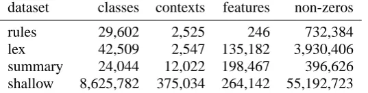
dataset classes contexts features non-zeros

[image:5.595.174.443.72.140.2]

rules 29,602 2,525 246 732,384 lex 42,509 2,547 135,182 3,930,406 summary 24,044 12,022 198,467 396,626 shallow 8,625,782 375,034 264,142 55,192,723

Table 1: Datasets used in experiments

of stochastic attribute value grammars, one with a small set of SCFG-like features, and with a very large set of fine-grained lexical features (Bouma et al., 2001). The ‘summary’ dataset is part of a sentence extraction task (Osborne, to appear), and the ‘shallow’ dataset is drawn from a text chunking application (Osborne, 2002). These datasets vary widely in their size and composition, and are repre-sentative of the kinds of datasets typically encoun-tered in applying ME models to NLP classification tasks.

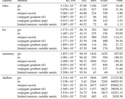
The results of applying each of the parameter es-timation algorithms to each of the datasets is sum-marized in Table 2. For each run, we report the KL divergence between the fitted model and the train-ing data at convergence, the prediction accuracy of fitted model on a held-out test set (the fraction of contexts for which the event with the highest prob-ability under the model also had the highest proba-bility under the reference distribution), the number of iterations required, the number of log-likelihood and gradient evaluations required (algorithms which use a line search may require several function eval-uations per iteration), and the total elapsed time (in seconds).2

There are a few things to observe about these results. First, while IIS converges in fewer steps the GIS, it takes substantially more time. At least for this implementation, the additional bookkeeping overhead required by IIS more than cancels any im-provements in speed offered by accelerated conver-gence. This may be a misleading conclusion, how-ever, since a more finely tuned implementation of IIS may well take much less time per iteration than the one used for these experiments. However, even if each iteration of IIS could be made as fast as an

2_{The reported time does not include the time required to}

in-put the training data, which is difficult to reproduce and which is the same for all the algorithms being tested. All tests were run using one CPU of a dual processor 1700MHz Pentium 4 with 2 gigabytes of main memory at the Center for High Per-formance Computing and Visualisation, University of Gronin-gen.

iteration of GIS (which seems unlikely), the bene-fits of IIS over GIS would in these cases be quite modest.

Second, note that for three of the four datasets, the KL divergence at convergence is roughly the same for all of the algorithms. For the ‘summary’ dataset, however, they differ by up to two orders of magnitude. This is an indication that the gence test in (6) is sensitive to the rate of conver-gence and thus to the choice of algorithm. Any de-gree of precision desired could be reached by any of the algorithms, with the appropriate value of ε. However, GIS, say, would require many more itera-tions than reported in Table 2 to reach the precision achieved by the limited memory variable metric al-gorithm.

Third, the prediction accuracy is, in most cases, more or less the same for all of the algorithms. Some variability is to be expected—all of the data sets being considered here are badly ill-conditioned, and many different models will yield the same like-lihood. In a few cases, however, the prediction accuracy differs more substantially. For the two SAVG data sets (‘rules’ and ‘lex’), GIS has a small advantage over the other methods. More dramati-cally, both iterative scaling methods perform very poorly on the ‘shallow’ dataset. In this case, the training data is very sparse. Many features are nearly ‘pseudo-minimal’ in the sense of Johnson et al. (1999), and so receive weights approaching−∞. Smoothing the reference probabilities would likely improve the results for all of the methods and re-duce the observed differences. However, this does suggest that gradient-based methods are robust to certain problems with the training data.

(6)

algo-Dataset Method KL Div. Acc Iters Evals Time

rules gis 5.124×10−2 47.00 1186 1187 16.68

iis 5.079×10−2 43.82 917 918 31.36

steepest ascent 5.065×10−2 44.88 224 350 4.80 conjugate gradient (fr) 5.007×10−2 44.17 66 181 2.57 conjugate gradient (prp) 5.013×10−2 46.29 59 142 1.93 limited memory variable metric 5.007×10−2 44.52 72 81 1.13

lex gis 1.573×10−3 46.74 363 364 31.69

iis 1.487×10−3 42.15 235 236 95.09

summary gis 1.857×10−3 96.10 1424 1425 107.05

iis 1.081×10−3 96.10 593 594 188.54

shallow gis 3.314×10−2 14.19 3494 3495 21223.86

iis 3.238×10−2 5.42 3264 3265 66855.92

[image:6.595.88.524.76.422.2]

Table 2: Results of comparison.

rithm performs substantially better than any of the competing methods.

4 Conclusions

In this paper, we have described experiments com-paring the performance of a number of different al-gorithms for estimating the parameters of a con-ditional ME model. The results show that vari-ants of iterative scaling, the algorithms which are most widely used in the literature, perform quite poorly when compared to general function opti-mization algorithms such as conjugate gradient and variable metric methods. And, more specifically, for the NLP classification tasks considered, the lim-ited memory variable metric algorithm of Benson and Mor´e (2001) outperforms the other choices by a substantial margin.

This conclusion has obvious consequences for the field. ME modeling is a commonly used machine learning technique, and the application of improved

parameter estimation algorithms will it practical to construct larger, more complex models. And, since the parameters of individual models can be esti-mated quite quickly, this will further open up the possibility for more sophisticated model and feature selection techniques which compare large numbers of alternative model specifications. This suggests that more comprehensive experiments to compare the convergence rate and accuracy of various algo-rithms on a wider range of problems is called for.

(7)

Acknowledgements

The research of Dr. Malouf has been made possible by a fellowship of the Royal Netherlands Academy of Arts and Sciences and by the NWO PIONIER project

Algo-rithms for Linguistic Processing. Thanks also to Stephen

Clark, Andreas Eisele, Detlef Prescher, Miles Osborne, and Gertjan van Noord for helpful comments and test data.

References

Steven P. Abney. 1997. Stochastic attribute-value grammars. Computational Linguistics, 23:597– 618.

Satish Balay, William D. Gropp, Lois Curfman McInnes, and Barry F. Smith. 1997. Efficienct management of parallelism in object oriented nu-merical software libraries. In E. Arge, A. M. Bru-aset, and H. P. Langtangen, editors, Modern Soft-ware Tools in Scientific Computing, pages 163– 202. Birkhauser Press.

Satish Balay, Kris Buschelman, William D. Gropp, Dinesh Kaushik, Lois Curfman McInnes, and Barry F. Smith. 2001. PETSc home page.

http://www.mcs.anl.gov/petsc.

Satish Balay, William D. Gropp, Lois Curfman McInnes, and Barry F. Smith. 2002. PETSc users manual. Technical Report ANL-95/11–Revision 2.1.2, Argonne National Laboratory.

Steven J. Benson and Jorge J. Mor´e. 2001. A lim-ited memory variable metric method for bound constrained minimization. Preprint ANL/ACS-P909-0901, Argonne National Laboratory. Steven J. Benson, Lois Curfman McInnes, Jorge J.

Mor´e, and Jason Sarich. 2002. TAO users manual. Technical Report ANL/MCS-TM-242– Revision 1.4, Argonne National Laboratory. Adam Berger, Stephen Della Pietra, and Vincent

Della Pietra. 1996. A maximum entropy ap-proach to natural language processing. Compu-tational Linguistics, 22.

Gosse Bouma, Gertjan van Noord, and Robert Mal-ouf. 2001. Alpino: wide coverage computational analysis of Dutch. In W. Daelemans, K. Sima’an, J. Veenstra, and J. Zavrel, editors, Computational Linguistics in the Netherlands 2000, pages 45– 59. Rodolpi, Amsterdam.

Zhiyi Chi. 1998. Probability models for complex systems. Ph.D. thesis, Brown University.

J. Darroch and D. Ratcliff. 1972. Generalized it-erative scaling for log-linear models. Ann. Math. Statistics, 43:1470–1480.

Stephen Della Pietra, Vincent Della Pietra, and John Lafferty. 1997. Inducing features of ran-dom fields. IEEE Transactions on Pattern Analy-sis and Machine Intelligence, 19:380–393. W.E. Deming and F.F. Stephan. 1940. On a least

squares adjustment of a sampled frequency table when the expected marginals are known. Annals of Mathematical Statistics, 11:427–444.

Elizabeth D. Dolan and Jorge J. Mor´e. 2002. Benchmarking optimization software with per-formance profiles. Mathematical Programming, 91:201–213.

Mark Johnson, Stuart Geman, Stephen Canon, Zhiyi Chi, and Stefan Riezler. 1999. Estimators for stochastic “unification-based” grammars. In Proceedings of the 37th Annual Meeting of the ACL, pages 535–541, College Park, Maryland. John Lafferty and Bernhard Suhm. 1996. Cluster

expansions and iterative scaling for maximum en-tropy language models. In K. Hanson and R. Sil-ver, editors, Maximum Entropy and Bayesian Methods. Kluwer.

John Lafferty, Fernando Pereira, and Andrew Mc-Callum. 2001. Conditional random fields: Prob-abilistic models for segmenting and labeling se-quence data. In International Conference on Ma-chine Learning (ICML).

Thomas P. Minka. 2001. Algorithms for maximum-likelihood logistic regression. Statis-tics Tech Report 758, CMU.

Jorge Nocedal and Stephen J. Wright. 1999. Nu-merical Optimization. Springer, New York. Jorge Nocedal. 1997. Large scale unconstrained

optimization. In A. Watson and I. Duff, editors, The State of the Art in Numerical Analysis, pages 311–338. Oxford University Press.

Miles Osborne. 2002. Shallow parsing using noisy and non-stationary training material. Journal of Machine Learning Research, 2:695–719.

Miles Osborne. to appear. Using maximum entropy for sentence extraction. In Proceedings of the ACL 2002 Workshop on Automatic Summariza-tion, Philadelphia.

Adwait Ratnaparkhi. 1998. Maximum entropy models for natural language ambiguity resolu-tion. Ph.D. thesis, University of Pennsylvania. Jun Wu and Sanjeev Khudanpur. 2000. Efficient