A production inventory model with exponential demand rate and reverse logistic Pages 521-542 Download PDF

(1)

International Journal of Industrial Engineering Computations 5 (2014) 521–542

Contents lists available at GrowingScience

International Journal of Industrial Engineering Computations

homepage: www.GrowingScience.com/ijiec

A production inventory model with exponential demand rate and reverse logistics

Ritu Raja*, Naresh Kumar Kaliramana, Shalini Chandrab and Harish Chaudharyc

a

Research Scholar, Centre for Mathematical Sciences, Banasthali University, P.O. Banasthali Vidyapith, Rajasthan-304022, India

b

Associate Professor, Centre for Mathematical Sciences, Banasthali University, P.O. Banasthali Vidyapith, Banasthali – 304022, Rajasthan, India

c

Assistant Professor, Department of Management Studies, Indian Institute of Technology, Delhi, New Delhi-110016, India C H R O N I C L E A B S T R A C T

Article history: Received January 6 2014 Received in Revised Format June 15 2014

Accepted July 17 2014 Available online July 31 2014

The objective of this paper is to develop an integrated production inventory model for reworkable items with exponential demand rate. This is a three-layer supply chain model with perspectives of supplier, producer and retailer. Supplier delivers raw material to the producer and finished goods to the retailer. We consider perfect and imperfect quality products, product reliability and reworking of imperfect items. After screening, defective items reworked at a cost just after the regular manufacturing schedule. At the beginning, the manufacturing system starts produce perfect items, after some time the manufacturing system can undergo into “out-of-control” situation from “in-control” situation, which is controlled by reverse logistic technique. This paper deliberates the effects of business strategies like optimum order size of raw material, exponential demand rate, production rate is demand dependent, idle times and reverse logistics for an integrated marketing system. Mathematica is used to develop the optimal solution of production rate and raw material order for maximum expected average profit. A numerical example and sensitivity analysis is illustrated to validate the model.

Imperfect Production Reverse Logistics Integrated Supply Chain

1. Introduction

(2)

Liu and Yang (1996) investigated a particular stage manufacturing setup with defective method of supplying of reworkable and non-reworkable objects. The impact of imperfect objects on the batch sizing procedure was renowned in the works of Sana et al. (2007, 2007a), with others. Kim and Hong (1999) considered that imperfect objects could be found after the manufacturing run and the imperfect objects were reworked at a rate. Banerjee and Kim (1995) considered the integrated inventory models in which the retailer and customer coordinate their manufacturing and ordering plan, in order to lesser the common inventory costs.

Khouja and Mehrez (1994) considered three coordination systems among the members of the supply chain and showed that several coordination systems could induce to significant decrease in total price. Cardenas-Barron (2007) extended the model of Khouja and Mehrez (1994) by mathematical method, assuming n-stage multi-customer supply chain inventory coordination. Jalbar et al. (2008) developed a multi-echelon inventory coordination in which one retailer delivers an item to many customers. Chiu (2003) developed an economic production quantity model with backorders by combining the assumptions of a symmetrical of the imperfect objects were reworked to build them superior quality objects instead of reworking on all the imperfect objects and the remaining objects are sold at a low rate. Yang and Wee (2001) developed a supply chain model by integrating producer, distributer and vendor as three members of the chain.

Cardenas-Barron (2008) presented a straightforward derivation to discover best production lot size with rework procedure at solitary phase manufacturing method. Cardenas-Barron (2009) developed an economic production quantity model with planned backorders for determining the manufacturing batch size and the size of backorders in an imperfect production process where all imperfect objects were reworked at the similar rotation. Sana and Chaudhuri (2010), Sana (2010, 2010a), Sarkar et al. (2010) and Chiu et al. (2007) showed that the imperfect objects might be reworked at a cost where overall production-inventory costs could be decreased considerably.

Chiu et al. (2007) developed the job of Chiu (2003) and considered the best run-time difficulty of economic production quantity model with scrap, reworking of imperfect objects and stochastic breakdowns. Sarker et al. (2008) addressed the problem connecting to reworking of imperfect objects in a multi-stage manufacturing method by considering two operational policies: reworking of imperfect objects within the same cycle and after N cycles. Biswas and Sarker (2008) described an inventory system of a solitary manufacturing procedure with an in-cycle rework strategy of fragment with complete analysis. Sana (2011) developed an integrated production inventory model of perfect and imperfect quality products in a three-layer supply chain.

Jamal et al. (2004) developed a manufacturing system with rework process consisting two cases of rework process to minimize the total production cost. At the first instant, they executed reworking in the same cycle. At the second instant, they executed reworking after N cycles. Chiu et al. (2007) considered a manufacturing system with rework, including optimal lot sizing decision, random scrap rate and service level constraint. They derived that the expected total cost of a manufacturing system is less if backlogging is allowed or equal if backlogging is not allowed. Hafshejani et al. (2012) presented a multi-product economic production quantity model with imperfect quality items and reworking, it is a nonlinear programming problem solved by genetic algorithm with limited warehouse space.

(3)

R Raj et al. / International Journal of Industrial Engineering Computations 5 (2014)

allowed and waiting time for imperfect quality item. Peter Chiu et al. (2010) developed a mathematical model to establish the optimal run time for a defective fixed production rate with rework, scrap and stochastic machine wreck. Wee and Chung (2009) and Chung and Wee (2010) developed an integrated production inventory model with deterioration assuming rework and green component value design. They extended the economic production quantity model with product reliability. We developed a mathematical model of three–layer supply chain including supplier, producer and retailer. The imperfect items at retailer’s level are sent back to the external supplier and the imperfect items at producer’s level are reworked after regular manufacturing time. The average profit of producer at in-control situation and out-of-in-control situation is considered to derive the solution of the problem. The average profits of suppliers and retailers are considered also.

2. Essential assumptions and symbolizations

The mathematical model is developed on the bases of following assumptions:

1. The demand rates are exponential increasing function of time for each member of three layer supply chain.

2. Production rate is demand dependent i.e. P t

 

D t

 

, where

 

at 1

D t be and  

3. Production cost per unit item is production rate dependent. 4. Idle time costs are assumed at supplier’s and producer’s level.

5. Different probability distributions functions are considered for defective items at supplier’s level. 6. Single item products are considered for joint effect of supplier, producer and retailer in a three layer supply chain.

7. Replenishment rate is instantly infinite but its size is finite at supplier’s level. 8. Stock-out situation is not conceded.

9. No product of producer is discarded at any stage. 10. No imperfect items are manufactured during rework.

11. Reworking starts just after the regular production process in each production run. 12. The imperfect objects are restored to its original quality, after reworking.

13. Insignificant lead time.

The mathematical model is developed on the bases of following symbolizations:

 

s

Q t Supplier’s on-hand inventory of good items at time t,

 

p

Q t Producer’s on-hand inventory of good items at time t,

 

r

p

(4)

 

r

Q t Retailer’s on-hand inventory of good items at timet,

R Supplier’s replenishment lot size,

at

be

 Producer’s production rate that is equal to supplier’s demand rate,

 _{Supplier’s proportional probability of imperfect items with probability density function}_f

_{ }

_ _,

s

A Supplier’s set up cost,

s

r Supplier’s screening rate per unit time,

c

S Supplier’s screening cost per unit item,

s

h Supplier’s holding cost per unit per unit time,

s

I Supplier’s cost per unit idle time,

s

C Supplier’s purchasing cost per unit item,

s

w Supplier’s selling price per unit perfect items,

s

w Supplier’s selling price per unit imperfect items,

 

E x Expected value of variablex, SAP Supplier’s average profit,

ESAP Supplier’s expected average profit,

 The percentage of imperfect items in “out-of-control” situation at producer level, 1

at

be

 Rate of reworking per unit time,



Random time with mean 1

 after which the production system becomes uncontrollable for

producer,

 

F  Probability distribution function of,

 

f  Probability density function of,

p

A Producer’s set up cost,

p

r Producer’s screening rate per unit time,

p

S Producer’s screening cost per unit item,

p

h Producer’s holding cost per unit per unit time for perfect items, '

p

h Producer’s holding cost per unit per unit time for defective items, which would be reworked,

'

p

r Cost to rework for imperfect item of producer,

L Cost of labor, energy, technology at fixed rate,

 _{Cost of tool and die is a variation constant,}

I

p Producer’s cost per unit idle time,

 

C P Per unit item production cost,

N Numbers of imperfect objects in the production process,

p

w Producer’s selling price per unit perfect item,

p

w Producer’s selling price per unit imperfect item, PAP Producer’s average profit,

EPAP Producer’s expected average profit,

at c

be Customer’s demand rate,

at r

(5)

r

A Retailer’s set up cost,

r

h Retailer’s holding cost per unit per unit time,

r

w Retailer’s selling price per unit item,

RAP Retailer’s average profit,

ERAP Retailer’s expected average profit,

T Retailer’s cycle length.

Material Supply

Supplier's Producer's Retailer's Customers

Demand Demand Demand

Product

Warehouse _Warehouse _Warehouse

The Integrated Material Run

Raw Finished

Fig. 1. The integrated material run 3. Mathematical Model

In this projected model, supplier delivers the raw materials at rate__beat_{to the producer up to}

manufacturing run timet₁. The imperfect objects at supplier level are sent back after examine carefully with sale rate w_s per unit item to the external dealer from where the raw materials are purchased. We assumed that the manufacturing process is “in-control” state at starting stage. The process may shift to an “out-off-control” state and may produce imperfect objects after a random time

 

 with mean 1



 

 

 . The total imperfect objects manufactured at time t₁ are reworked with production rate be₁at, which takes timet_r.The inventory fills up after accommodating the demand at

r

be of retailer during manufacturing run timet₁. The customers demand is fulfilled with rate be_cat by retailer where the delivery charge of produced items is sustained up to timekT k



1



. The assembled inventory at time

kT decreases and accomplishes to zero level at timeT. The leading differential equations at supplier, producer and retailer level are as follows:

3.1. Supplier’s specific average profit

The leading differential equation is

 

s at

dQ t

be dt  

(1)

(6)

 



1





1



, 0 1

at s

b

Q t e R t t

a





      (2)

We have Q tS

 

₁ 0





1

1 1

log 1 a R

t

a b

 

  

  _  _

 

(3)

The inventory cost of perfect objects is



1



log 1



1





1



s a R

h b

IC R R

a a b

 

 



_ _    

         

 

   

 

(4)

Inventory cost of defective objects is 2

S i

s

h R

IC r



 (5)

Idle Time

t1

Time R

Supplier Z Q

where Q = R Z = R – beat

Fig. 2. Trend on inventory change

The price of screening isS R_c . The earning from selling the perfect and imperfect items is







ws 1 RwsR



. The buying price of Robjects isC Rs . The price of establishment isAs. The idle

time cost isI T_s

_

t₁

_

. The supplier’s average profit is, using t₁ 1log 1 a



1



R

a b

 

  

 _  _

 

























2 1

1 1

1 log 1

1 1

1 log 1 1

s s c s s

s

s s

a R

SAP w R w R S C R I T

T a b

a R

h b a R

R R A

T a a b r



 





 

 



    

       _    _

   

 

 __ _    _ 

            

 

     

 

(6)

3.2. Producer’s specific average profit

If a manufacturing process does not perform well according to process designer’s specification then it is said to be “out-of-control”. The constraint



is a design variable and an indicator of manufactured goods consistency. Consistency of machines in a production system is usually authenticated to be an exponential function of time t which isR t

 

et

(7)

Here

_{ }

0

t

F t 

_

f u du, where f t

 

is the failure probability density function then

_{ }

0

1

f t dt







.

Thus

_{ }

d



_{ }



t

f t F t e

dt

  

 

The unit production cost is

 

at

s at

L

C P w be

be 



   (7)

We assumed that the manufacturing process is in “in-control” state at starting stage. The process may shift to an “out-off-control” state and may produce imperfect objects after a random time

 

 with mean 1



 

 

 

. The holding cost per unit per unit time for defective items is greater than the holding cost per unit per unit time for perfect items. Two cases are gets up in this operating system:

3.2.1 Case I: When0  t₁, the “out-of-control” state exists during operations time. At the beginning, the production rate is__beat_{. The inventory fills up after accommodating the demand} at

r

be

of retailer during manufacturing run timet₁. Thus

 

 exists in the time period



0,t₁



, the perfect items are produces during



0,



and it produces both perfect and imperfect items during



,t₁



. The total numbers of items manufactured during

_

0,t₁

_

are used to fulfill the demand for the time duration



t1t2



. Since, the total numbers of imperfect objects manufactured at time t1 are reworked with manufacturing rate _be₁at

 which takes timet_r. The timet₃ is necessary to sell out the reworked items. On-hand inventory of perfect items at time t can be illustrated by the following differential equations:

 

p at at

r

dQ t

be be

dt  

(8)

withQp

 

0 0, 0 t



 



1



p at at

r

dQ t

be be

dt    

(9)

withQ_p

_{ }

 



beat be_rat



,   t t₁

 

p at

r

dQ t

be

dt  

(10)

withQ_p

 

0 Q t_p

 

₁ andQ t_p

 

₂ 0, 0 t t₂ From Eq. (8), we have

 



1 at





1 at



, 0

p r

b b

Q t e e t

a a





 

      

 

(11)

(8)

 

















1

,

at at at a a at

p r r r

b _b

Q t b e e e e e e t t

a a

 

 

   

        ₍₁₂₎

From Eq. (10), we have

 

_

1 1

_





_

1

_

_

1

_

2 1

1 , 0

at at at a at a at

p r r r r

b b

Q t b e e e e e e e t t

a a

 

 

  

          (13)

Now,Q_p

 

t₂ 0 We have





1





1





2 1

log 1 _rat 1 at 1 a _ra 1

t a e a e e e

a

 

     

 

 _         _

Using t₁ 1log 1 a



1



R

a b

 

  

 _  _

 

, we have





















2

1 1

log 1 1 1 a R 1 a _ra 1

t a a e e

a b

 



     



    

            

   

 

(14)

The inventory level Q t_r

 

of defective items at time t liquidates the following differential equations:

 

p at

dQ t

be

dt 

(15a)

withQp

 

 0,   t t1

 

p at

r

dQ t

be

dt  

(15b)

with

 

0

 

₁ at



₁



p p

Q Q t be t  andQ_p

 

t₃ 0,0 t t₃

From Eq. (15a) and Eq. (15b), we have

 



1



1 ,

at a

p

b

Q t e e t t

a

 



    (16)

 



1







3 1 , 0

at a at

p r

b b

Q t e e e t t

a a

 

      (17)

Thus, Q_p

 

t₃ 0





3

1 1

log 1 1 a R a

t e

a b

 





   

      

  

 

(9)

Here, kT t₁t₂t₃





























1

1 1 1

1 1

1 1 1

log 1 1 1 a a r a a R a a b a R

b a R

e e kT b a a R e b            _                                              _ _ _ _ _   _ _  __       __ _ _ ___  _  _   _        (19)

Thus, the inventory cost for perfect objects is

























1 1 1

1 1 1 1

2 1

1 2

1 2 2 2

2

2 2 2

1 1

1

at at at

a a a a a

r r r r r

at a a a at a at at

p p r

at a at

r r r

b b

at e e a e a e a e e e e

a a

b

HG h e at e e e at e at e b e e t

a b

e e t e t t

a a                                           _        _     _ _ _ _     _ _    (20)

Inventory cost of defective objects is



























1 1 1

3

1

1 1

2 2

1 3 1 2

2

3

' ' 1

1

r

at a a at at a at

p p r r r

at at at

r r r

p

at a

b b

HG h e e a e at e at e at e e at

a a

b b

e e t t be t t t

a a

h

b

e e t

a                 _         _                  _ _      (21)

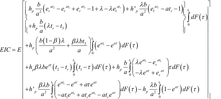
Adding Eq. (20) and Eq. (21), the total inventory cost is









_

_































1 1 1

1 2

1 1 1

3 1

2

1 1

2 2

1 3 1 2

2 1 1 ' 1 1 r r

at at a a at a a

r r

p

at at

r r

at a a at at a at

p r r r

at at at at a

p r r r

a e e e e e e e

b

TIC h

a _e _e

b b

h e e a e at e at e at e e at

a a

b b b

h e e t t be t t t e e

a a a

                        _ _ _ _ _ _ _ _             _         _  

 _           t₃_

 

(10)













 









 



 



 

3

2 1

1

1 1

1 1 1 1

1 1

2 2

0 3

3 2

0

2 1

0 0

1 ' 1

1

'

r r

at

at at at at

t

p r r r p r

p r

t

at a

p

t t at at

r at

p r p _a _a

r

p

b b

h e e e e h e at

a a _dF

b

h t t

a

b bt

h e e dF

EIC E a a

e e

b

h be t t t dF h dF

a e e

h



 

  

 

  





    

 

 

       

 

 

_ _ 

 

 

  

 _  _ 

 _ _

  

    _ _

 

 





 





 

1 1 1

1 1

2 2

0 1 0

1

t at a a t

a p

at at a

r r

e e a e

b b

dF h e dF

a at e at e at e a

 

 

 

 

 

 

   

 

 

 _ _ 

  

   







Thus, TIC is a function of random variable



and t₁ depends on random variable



. The expected number of imperfect objects in a manufacturing lot size



1



Ris as follows,

 





 





1 1

1

1 1 2 2

0 0

1 1

t t

t

at at at t

E N be t dF be t ed be e

      

  



  

     _   _

 



Expand the function _et1 up to third term, we have

 

2

1 1

2

at

E N  be t (22)

Total expected rework cost is

 

2

1 1

2

at

p p

r E N  r be t (23)

The cost of arrangement isA_p

The income from selling the perfect and imperfect items is

Idle Time

kT Time

O

n

-h

an

d

I

n

v

e

n

to

ry

Q

where Q = (1 – bea t

Z = – ber at

t_r t₂ t₃

r Z

Fig. 3. The change in inventory







₁ 1 1







₁



₁



1

at at akT

p s p s r

w  be wbe w w  b   e



 

  _  _   



(11)

The cost of screening is 1 1



_

₁

_

₁



1

at akT

p p r

S be S b   e



   



In this case,

Total expected profit =









 









 













 





 





_

_

 

1 1

3

2 1

1 1 1

1

0 0

1 1 3

2 2

3

2 2

0 0 0

2

1 1

1

1 ' 1

1 1

r r

t t

akT

p s r I p

at

at at at at

p r r r p r p r

t t t

at

a a

p p

at p

w w b e dF p T kT A dF

b b b

h e e e e h e at h t t

a a a

b bt

b

E dF h e dF h e e dF

a a a

h be t t

 



   





  

  



  



 

      

 



 

 

_           _

 

  

      

 

 





 



 

_

_

 













 





 

1 1

1

0 0

1 1

2

0 0

'

1 1

t t

at at a a

r p r r

t t

p a at at

r r p

b

t dF h e e e e dF

a

h b

a at e at at e dF r be t dF

a

 



     



    

 

 

      

 

_ _ _ _ _ _ _ _ 

 

 



(24)

3.2.2 Case II:

Whent₁   , the system is in “in-control” state during manufacturing process The leading differential equations are as follows:

 

p at at

r

dQ t

be be

dt  

(25)

with Qp

 

0 0, 0 t t1

 

p at

r

dQ t

be

dt  

(26)

with Q_p

 

t'₂ 0 and

_{ }

0



at at



₁

p r

Q  be be t , 0 t t'₂ From Eq. (25) and Eq. (26), we get

 



1





1



, 0 1

at at

p r

b b

Q t e e t t

a a



 

_    _  

 

(27)

 



1





1







2

1 at 1 at 1 at , 0 '

p r r

b b b

Q t e e e t t

a a a



        (28)

Thus,Qp

_{ }

t'₂ 0





1 1

2 1

' log 2 _rat 1 at

t e e

a   

(12)

Idle Time

kT Time

O

n

-h

a

n

d

I

n

v

en

to

ry

Producer Z Q

where Q = (1 – beat

Z = – be_ra t tr t2

Fig. 4. The change of on-hand inventory Inventory cost for perfect objects is





1







1

_

1

_



'2

1 2

1 1 1

1 at 2 2 at 1 at ' at

p r r r

b

IC h t e e e t e

a  a a   a

   

 _  _  _       _

 

 

Using Eq. (29), we get





















1

1 1 1 1

1

1 1

1 2

1

1 1 log 2 1

at r

p

at at at at

r r

t e

b a a

IC h

a

e e e e

a

 

   

 _  _ 

 

 

 



 _ _

      

 _ _

 

Here, rework cost is zero.

Total expected profit









































 

1

1 1 1 1

1

1 1

1

1 1

1 2

1

1 1 log 2 1

akT

p s r I p

at r t

p

at at at at

r r

w w b e p T kT A

E _t _e dF

b a a

h a

e e e e

a



 





 



    

      

    



 

   

  _ _ _ _ 

 _ _ _ _ _ _ _ _

 

 

 _    

 

   

 

          

 

    

 



(30)

(13)









 









 













 





 









 

1 1 3 2 1 1 1 1 0 0 1 2 1 3 2 2 0 0 3 2 0 1 1 1 1 ' 1 1 1 r r t t akT s

p r I p

p at at at at

r r r

p at p

r r t t p a t at a p w

w b e dF p T kT A dF

h b

e e e e

a

h b h b

e at t t

a a

h b

dF e dF

EP E _a

b bt

h e e dF

a a                       _  _ _{ } _ _ _                      _ _ _ _ _                  





 



 





 









 





 

1 1 1 1 1 1 1 1 2 1 0 0 1 2

0 1 0

1 ' 1 1 1 t t at at

at a a

p r p r r

a t t r p at p at r p s b

h be t t t dF h e e e e dF

a

a at e

h b

dF r be t dF

a at at e

w w b

E                                                      _ _ _ _ _ _ _           _ _                            











































 

1 1

1 1 1 1

1

1 1

1 2

1

1 1 log 2 1

akT

r I p

at r t

p

at at at at

r r

e p T kT A

dF

t e

b a a

h a

e e e e

a                            _ _ _ _    _  _  _  _     _                                



(31)

Thus, we have

_

_

_{ }

_

_





1 1

1

2 2 2 1

1 1 1 2

0 0 2 2 1 t t t t

t  dF   t  ed t e

 

 

      



. Expand the function

1

t

e up to fourth term, we have





 

1 3 2 ₁ 1 0 3 t t

t  dF  



. Thus, the average expected profit of the producer is  





 



 



 









   





   





1 1 3 2 1 1 1 1 0 0 1 2 2 0 0 1 3 2 3 2 1 1 1 1 1 ' 1 1 1 r r t t akT s

p r I p

p at at at at

t t

r r r

p a

p at p

r r

at a

p

w

w b e dF p T kT A dF

h b

e e e e

h b

a _dF _e _dF

h b h b a

e at t t

a a

b bt

EPAP h e e dF

T a a

                                                      _ _ _ _           _  _   



           





 





  1 1 1 1 1 1 1

1 1 1

1 0 0 2 1 0 0 1 2 0 ' 1 1 t t at p t t

p at at

at a a

p r r r

t

at a a at at a

p r r

p s

r be t dF

h b

h be t t t dF e e e e dF

a b

h e e a e at e at e at e dF

a w w T                                           _ _ _                    _ _ _ _ _ _                   



 







 



   













  1 1

1 1 1 1

1

1 1

1 2

1

1 1 log 2 1

akT

r I p

at r t

p

at at at at

r r

b e p T kT A

dF

t e

b a a

h a

e e e e

(14)

3.3. Retailer’s specific average profit.

The leading differential equations are

 





r at at

r c

dQ t

b e e

dt  

(33)

with Qr

 

0 0 ,0 t kT and

 

r at

c

dQ t

be

dt  

(34)

with Q Tr

_{ }

0,kT t T From Eq. (33) and Eq. (34), we have

 



at at



, 0

r r c

b

Q t e e t kT

a

    (35)

and using

_

_



akT akT



r r c

b

Q kT e e

a

 

 



akT at



,

r r c

b

Q t e e kT t T

a

    (36)

Thus,

_{ }

0 1

at c

r at

r

be

Q T k

be

    as at at

r c

e e

For possibility of the model, t₁kTT must be gratified. As stated, kTT grasps ask1. Now, we have t₁kT













1 1

1

1 1

at

at at at at

r r

at r

be t

t e e E e e

be

 

   



       (37)

O

n

-h

an

d

I

n

v

en

to

ry

Z Retailer

T

where Z = –be_ca t

(15)

The cost of arrangement is A_r

The income from selling items isw be T_r _cat The cost of buying objects isw be T_p _cat . The cost of inventory is

 

2









0

2 1

kT T

akT aT akT

r r r r r c c r

kT

b

H h Q t dt Q t dt h e e e aT akT a

 

 _  _    







(38)

The retailer’s average profit is









2 1

at at akT aT akT

r c r p c r c c r

b

RAP w be T A w be T h e e e aT akT

T a

 

 _        _

 

(39)

3.4. Leader-Follower Association

Producer is the leader; supplier and retailer are the followers. From Eq. (32), usingt₁ 1log 1 a



1



R

a b

 

  

 _  _

 

, akt at

r c

be be and T 1 log 1 a

_

1

_

R

ak b 

 

 _   _

 

The producer’s expected average profit is

E [PAP] =





log 1 1

ak a

E R

b 

 

 

 

 _ _ 

 

 _ _

 

 





 





















2 2

2

2 2

2

2 2

1

2

1

1 log 1 1

1 log

p p

p p p p

p p

p p p

p

p p I

p p p I

h a E

h b

b w w S C P A R

r r

h h h b

w w S C P aE R

a a r

bh h _p _a

E R E R

a a ak b

bh h h b p

E R

a a a a

 



 



 

 



 



   

 

     

 

 _ _ 

   

 

    

 

   _   _   

 

   

 

   

_    _ _   _

 

 

 

_     _

 



1



1 aE R

b

 

 

 

 _ _ _ 

 _ _ _ 

 _ _ 

 

2

[ ] [ ( ) log(1 ) ( ) log(1 )]

log(1 )

P

E PAP M KSR HR J LR G NR F LR D B AR

NR

 

_ _           



 

(40)

where Pak , N aE

_

1

_

b 

  ,D hp ₂ b

a



 , _B pI

a

 , A aE



1



b

 



 ,J bh₂p

a

 ,F bh₂p

a 

(16)

 

p

p p p p

p

h b

M b w w S C P A

r           _     _       

, L hp E

_

1

_

a 

  ,SaE



1



 





2 2

2

p p p

p

h h h b

K w w S C P

r a a             _   _          

, _G pI

ak  ,





2 2 1 p p

h a E

H

r

 



From Eq. (6), usingt₁ 1log 1 a



1



R

a b       _  _  

, be_rakt be_cat and T 1 log 1 a



1



R

ak b 

 

 _   _

 

The supplier’s expected average profit is













 









 













2 1 1 1

log 1 1 log 1 1

1 1

1 log 1

s

s s c s s

s s

s s s

h

E Rw E Rw R S C E R A

a

aE R

ak a

E SAP I E R

a r ak b

E R

b _b _aE _R

h E Rh I

a a b

             _ _ _ _ _ _ _          _ _        _   _        _ _   _{ } _  _ _  _ _ _ _ _ _ _ _    _ _  _  _ _      (41)

From Eq. (39), using t₁ 1log 1 a



1



R

a b       _  _  

, akt at

r c

be be and T 1 log 1 a

_

1

_

R

ak b 

 

 _   _

 

The retailer’s expected average profit is





















1 1

log 1 1

r r

r p

h akA

E RAP w w k b aE R

a a E R b     _    _        _ _     (42) Solution:

For optimum value of EPAP [R], we have











 







2 2

2 log(1 )

( ) log

log(1 )

log(1 ) ( ) log

log 1 log 1

log(1 )

KS HR L NR

EPAP P

F D B LR A

R NR

L AR J LR G N

M KSR HR F D B LR

PN

AR J LR G NR

NR       _ _ _ _ _                               _ _

We consider EPAP 0

R





 , which give us the value of R













2 2 2

( log log ) ( log log )

log log ( log log log

log log log )

( log log )

H L N L A NH L N NL A

H L N L A NM KG F N D N B N

K A D A N A

R

NH L N NL A

      

       

  



  