Abstract— The FDV method was originally developed by T.J. Chung [3]-[6]. The authors developed and presented a modification to this method named MFDV method in [2]. The aim of this modification was to give the implicitness parameters a deeper physical meaning while maintaining the solution stability and robustness. In the present work the modified flowfield dependent variation method (MFDV) has been tested and verified for the solution of supersonic internal flow problems. Starting from compressible Euler flow equations and applying the MFDV method with finite element discretization, many successful supersonic internal flow problems have been reported. Special attention has been given to complex shockwave patterns. Finite element implementation has been carried out via standard Galerkin method. Good agreement has been obtained in all cases with available analytical solutions, if any, and published literatures.
Index Terms— Computational Fluid Dynamics (CFD), Flowfield Dependent Variation (FDV) method, Euler equations, Finite Element (FE), Galerkin method, Modified Flowfield Dependent Variation (MFDV) method.
I. NOMENCLATURE
i
a w wF Ui convection Jacobian tensor
v
c specific heat at constant volume
e static internal energy
t
e total internal energy
F convection flux
,
i j co-ordinate dimension counters = 1,2
*
L element characteristic length
M Mach No.
i
n boundary normal vector
P pressure
R gas constant
1
s 1st order convection FDV implicitness parameter
2
s 2nd order convection FDV implicitness parameter
T temperature
t time
¹ Professor, [email protected].
² The other two authors miss the late soul forever. ³ Research/Teaching Assistant, [email protected].
t
' time step
i
u velocity components in 2-D space
U conservation variables vector
i
x space co-ordinates
,
D E nodal element counters
= 1,2,3,4 for quadrilateral elements
) domain shape functions
) boundary shape functions
J specific heat ratio
gradient of a scalar function
U density
: domain boundary
* contour boundary
II. INTRODUCTION
The problem of internal supersonic flow has the potential of being investigated endlessly. To accurately calculate the flow properties in such flows, the solution technique should be able to handle the strong interactions resulting from any compressible flow phenomena like shockwave/expansion fan patterns in the solution domain, so in the recent decades many CFD research efforts ([2]-[9][10]) were directed towards the development of such numerical techniques. These techniques should be able to operate on flow domains with shockwaves without altering the solution accuracy. The authors presented the MFDV method for the first time in [2] and claimed that MFDV method is able to operate on different flow situations without losing its robustness or accuracy. So they want to demonstrate some of the MFDV capabilities in this paper via its ability to handle supersonic internal flow problems.
A shortened formulation of the Euler equations with the MFDV method will be presented followed with the finite element discretization for the resulting equations. After that, a quick review for the supersonic flow boundary conditions is presented. The final section contains the numerical results for three supersonic internal flow problems.
III. EULER EQUATIONS IN 2-DSPACE
The system of compressible Euler flow equations can be written in the conservation form as follows:
Solution of Supersonic Internal Flow Problems
Using MFDV
A. A. Megahed
¹, M. W. El-Mallah
², B. R. Girgis
³Engineering Mathematics and Physics Department,
Faculty of Engineering,
0 i i t x w w
wU wF (1)
Where; in 2-D space the conservation variables vector is given by:
>
U Uu1 Uu2 Uet@
U (2)
Also the convection flux is given by:
1 2
2
1 2 1
2
1 2 2
1 t 1 2 t 2
u u
u P u u
u u u P
u e Pu u e Pu
U U U U U U U U ª º « » « » « » « » ¬ ¼ F (3)
P URT (4)
v
e c T (5)
Eqn. (1) with the ideal gas equation of state Eqn. (4), and the thermally perfect gas assumption, Eqn. (5), completes the system of Euler’s flow equations.
Rewriting Eqn. (1) in a quasi-linear form as follows: 0
i i
t x
w w
wU a wU (6)
Where; ai is the convection Jacobian tensor1 which is considered to be time-step dependent.
IV. MFDVMETHOD FORMULATION
For a detailed step by step derivation of the MFDV method, the reader is referred to [1]. The MFDV method can be summarized in the following three steps:
A. Expanding n1
U around Un in a special form of Taylor expansion:
1 2 2 2 3
1
2 2
n s n s
n n t t O t
t t
w ' w
' ' w w U U U U Where; 1 1
1 0 1 1
n s n n
s s
t t t
w w w' d d
w w w
U U U
2
2 2 2 1
2 2
2 2 2 0 1
n s n n
s s
t t t
w w w ' d d
wU wU wU
1 1
n n n
'U U U
The implicitness parameters, s1 and s2 , are flowfield dependent. They may gain their physical meaning by being calculated from the flow variables’ fluctuations. The proposed formula by A. A. Megahed et al [2] for calculating s s1, 2 from the current flowfield is given by:
1 min ,1
s r (7)
2 1 1 1 2 s s (8)1 See the appendix for full listing of this Jacobian in 2-D space.
Where; *
min
r L M M , 0.05 K 0.2, and Mmin is the minimum Mach No. in the neighboring nodes (i.e. between the element nodes).
B. Substituting from Eqn. (6) into the Taylor expansion by interchanging the time derivatives with the spatial derivatives we get: 1 1 1 2 2 1 3 2 2 2 n n
n i i
i i n j i i j n j i i j t s x x t x x t
s O t
x x
§ w w' · ' ' ¨ w w ¸
© ¹
§w ·
' w
w ¨¨w ¸¸ © ¹
§w' ·
' w
w ¨¨ w ¸¸ '
© ¹ F F U F a F a (9)
C. Rewriting Eqn. (9) in the residual form and substituting all the ' terms with their Jacobian equivalents we get:
1 1 1 2 2 1 2 2 3 2 0 2 n n i i n i j i j n n j i ii i j
t s x t s x x t
t O t
x x x
w
' ' w '
' w
'
w w
§w · '
w w
' w w ¨¨w ¸¸ '
© ¹
U a U
a a U
F
F a
(10)
Rearranging Eqn. (10):
1 1 2 3 1 0n n n
i i
n n n
ij i j x O t x x w ' ' w w ' ' w w
U D U
E U Q
(11)
Where;
1 n
i 'ts i
D a ,
2
2 2 n
ij i j
t s
'
E a a , and
2 2
2
n n n
i i j
i i j
t t
x x x
'
w w
' w w w
Q F a F
Eqn. (11) can be solved either by finite difference methods or finite element methods. The latter has been chosen for two reasons; to take the well-known advantages of the finite element techniques, and to maximize the benefits from the gained physical meaning by the MFDV method.
V. FINITE ELEMENT DISCRETIZATION:STANDARD GALERKIN
METHOD
From the standard Galerkin method:
, d 0
) :
³
R U F (12)Where; R U F, is the residual of Eqn. (11)
In what follows the order of the solution error will be omitted for convenience. Expressing the conservation variables vector as a linear combination of the trial functions ) we have:
,t ) t
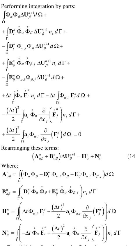
Performing integration by parts: 1 n d ) ) ' :
³
U 1 n ni n di
³
D ) ) 'U *1 ,
n n
i i d
³
D ) ) 'U :1 ,
n n
j
ij n di
³
E ) ) 'U *1 , ,
n n
ij "!i j ! d
#
$
³
E ) ) 'U :, n
n
i i i i
t % n d t d
%
&'&
( )
' )
³
F * ' )³
F :2 2 n j i i j t n d x * + + ,
' w § ·
) ¨ ¸ *
w © ¹
³
a F2
, 0
2
n
i i j
j t d x -. ' w ) : w
³
a FRearranging these terms:
n n n 1 n n/10 /10 0 / /
2
'
A B U H N (14)
Where;
, , ,n n n
i i ij i j d
314 34 3"4 3"4
5
) )
³
) ) ) ) :A D E
,
n n n
j i 687 ij 67 n di
697 :: :: ; § ) ) ) ) · * ¨ ¸ © ¹
³
B D E
2
, ,
2
n n n
i i i i j
j t
t d
x
< < <
=
§ ' w ·
¨ ¸
' )¨ ) ¸ :
w
© ¹
³
H F a F
2
2
n n
n
i i j i
j t
t n d
x
> >
>
?@? ? ?
A
§ ' w § ··
¨ ¸
' )¨ ) ¨ ¸¸ * w © ¹
© ¹
³
N F a F
Eqn (14) is referred to as the finite element equations. It is important to remember that by setting s1 0 and s2 1, the so called Taylor-Galerkin method is obtained. Actually, any known numerical scheme in either finite element or finite difference may rise as a special case of the FDV/MFDV methods with s1 and s2 fixed to certain values. For a comprehensive comparison between FDV and other methods the reader is referred to [6]. Allowing the implicitness parameters (s s1, 2) to vary from element to element gives the FDV/MFDV methods the ability to provide a unique and distinctive numerical scheme for each element according to its current flowfield properties.
VI. BOUNDARY CONDITIONS
It is well known that an efficient and robust boundary conditions implementation technique is a crucial issue for all CFD problems. In this section the most important boundary conditions are discussed. These boundary conditions are used to simulate many practical flow situations encountered in real supersonic internal flow problems.
A. Inviscid Wall Boundary Condition (No Penetration) There are many ways to implement the wall boundary conditions inside the Euler solver. One of the most successful methods is the method of co-ordinates rotation given in Reddy
[12] and implemented successfully by many others including F. Moussaoui [8], T. E. Tezduyar et al. [9]. In this method the velocity components at the solid wall are transformed to the normal and tangential components, as shown in Figure 1.
These axes are used to introduce the zero normal velocity (un 0.0) via equating the normal component to zero. The coordinate transformation matrix will take the form:
1 2 cos sin sin cos t n u u u u T T T T § · § ·§ · ¨ ¸ ¨© ¸¹¨ ¸
© ¹ © ¹
[image:3.612.45.277.46.469.2]For the nodes on the solid boundary a new vector of unknowns is to be introduced via the following rotation matrix:
Figure 1 Co-ordinates rotation at a solid wall
1 2
1 0 0 0
0 cos sin 0
0 sin cos 0
0 0 0 1
t n t t u u u u e e U U
U T T U
U T T U
U U § · § ·§ · ¨ ¸ ¨ ¸¨ ¸ ¨ ¸ ¨ ¸¨ ¸ ¨ ¸ ¨ ¸¨ ¸ ¨ ¸ ¨ ¸¨ ¸ © ¹
© ¹ © ¹
B. Supersonic Inlet Boundary Condition
From the theory of characteristics, all the flow properties should be defined in the supersonic inlet boundary condition. So, at the nodes on the supersonic inlet boundary the four flow properties (U U U U, u1, u2, et) are specified exactly.
C. Supersonic Exit Boundary Condition
Again from the theory of characteristics, all the flow properties should be extrapolated from the solution domain for the supersonic exit boundary condition. So, at the nodes on the supersonic inlet boundary the four flow properties (U U U, u1, u2,Uet) are left free. Another benefit from the finite element technique is that, no extrapolation technique is needed since the shape function assumed across the element will provide continuity of the unknowns at the boundary.
VII. NUMERICAL RESULTS
Many problems have been solved to validate the applicability and effectiveness of the MFDV method in the solution of supersonic internal flow problems. In all cases the method showed good agreement with analytical solutions, if any, and with the published literature. For more results using the MFDV
method, the reader is referred to [1] and [2]. All the test cases have been solved using FORTRAN 90 code and a preconditioned GMRES sparse matrix solver. The reader is referred to [13] and [14] for more details on GMRES. In this section we present three test cases.
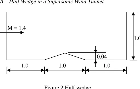
[image:4.612.54.300.122.278.2]A. Half Wedge in a Supersonic Wind Tunnel
Figure 2 Half wedge
The solution domain of a half wedge, as shown in Figure 2, is discretized uniformly with 120x80 bilinear rectangular elements. At the inlet boundary, the supersonic inlet boundary condition is used with the following values:
1 2
1.0, 1.40
0.0, t 2.76575
u
u e
U U
U U
On lower boundary and upper boundaries, the inviscid wall (no-penetration) boundary condition is used and the exit boundary is left free being supersonic exit.
Figure 5 shows the Mach No. contours. Our results match the results obtained from the oblique shockwave theory. Figure 6 shows the contours of s1 while Figure 7 shows the contours of
2
s . It is clear that s1 parameter resolves the solution itself and this interesting property for s1 may be utilized if an adaptation technique is to be used.
Figure 14 shows a comparison between the Mach No. at y = 0.5 from this test case and a relatively coarse grid (60x40). It is clear that as the grid gets finer the exact solution is approached. Also a higher over/under-shots can be observed for finer grids. This is due to the lost solution modes resulting from the grid selectivity.
B. Extended Compression Corner Problem
Figure 3 Extended compression corner
The extended compression corner problem is shown in Figure 3. The solution domain is discretized using 120x80 uniform bilinear quadrilateral elements. The inlet boundary is supersonic and the following values have been used:
1 2
1.0, 1.90
0.0, t 3.47855
u
u e
U U
U U
Again the no-penetration boundary condition is applied on both the upper and lower boundaries and the exit boundary is left free being supersonic.
Figure 8 shows the Mach No. contours. The shown results match very well the results of the analytical solution given from the oblique shock wave theory. Figure 9 shows the contours of
1
s and Figure 10 shows the contours of s2. Figure 15 is a comparison between the Mach No. at y = 0.5 from this test case and (60x40). The same trend that was observed at the first test case has, also, attained in this test case.
[image:4.612.314.548.286.420.2]C. Circular Arc Problem
Figure 4 Circular arc
The circular arc problem is shown in Figure 4. The circular arc maximum height is set to 0.04. The solution domain is discretized using 120x80 uniform bilinear quadrilateral elements. The inlet boundary is supersonic and the following values have been used:
1 2
1.0, 1.65
0.0, t 3.147
u
u e
U U
U U
[image:4.612.46.311.577.697.2]The no-penetration boundary condition is applied on both the upper and lower boundaries and the exit boundary is left free being supersonic.
Figure 11 shows the Mach No. contours. The shown results match very well the results given in [8] and [10]. Figure 12 shows the contours of s1 and Figure 13 shows the contours of
2
s . Figure 16 is a comparison between the Mach No. at y = 0.5 from this test case and a coarser grid (60x40). The same trend that was observed in the first and second test cases is observed in this test case also.
VIII. CONCLUSION
MFDV method is capable of recovering the implicitness parameters for the supersonic internal flow problems and it gave a satisfactory performance in all the tested problems. This work is regarded as an extension to the authors work in [1] and [2] to show the MFDV method ability to handle supersonic internal M = 1.4
0.04
1.0 1.0 1.0
1.0
0.8
1.0 1.0
1.0 1.0 M = 1.9
1.0 1.0 1.0
flows. The authors expect to publish another paper to validate the capabilities of MFDV in the solution of the subsonic/transonic flow problems very soon. Also they expect to publish an extension of the MFDV method to solve the Navier-Stokes flow equation in both the compressible and incompressible forms.
APPENDIX
The 2-D convection Jacobian, ai , is given by: 1
a
1
21 1 2
1 2 2 1
1 1
41 42 1 2 1
0 1 0 0 3 1 1
0 1
a u u
u u u u
a a u u u
J J J
J J
1 2 2
21 1 2
1
3 1
2
a J u J u
1 2 2
41 1 1 1 2 t
a u J u u Je
1 2 2
42 1 2
1 3 2 t
a Je J u u
2
a
1 2 2 1
2
31 1 2
2 2
41 1 2 43 2
0 0 1 0 0 1 3 1 1
u u u u
a u u
a u u a u
J J J
J J
2 2 2
31 2 1
1
3 1
2
a J u J u
2 2 2
41 2 1 1 2 t
a u J u u Je
2 2 2
43 1 2
1
3 2
t
a Je J u u
ACKNOWLEDGMENT
The authors would like to acknowledge Prof. T. J. Chung for his discussions regarding the original FDV method. Also the first and third authors want to express their deep sorrow for the pass away of the second author.
REFERENCES
[1] B.R. Girgis, Flowfield-Dependent Variation Method Applied to Compressible Euler Flow Equations, Master Thesis, Eng. Mathematics and Physics Dept., Cairo University, Giza, Egypt, 2007.
[2] A.A. Megahed, M.W. El-Mallah, B.R. Girgis, A modified flowfield dependent variation method applied to the compressible Euler flow equations, Eights Int. Congress of Fluid Dynamics and Propulsion, ICFDP8-EG-102, 2006.
[3] Chung, T.J., Transitions and interactions of inviscid/viscous, compressible/incompressible and laminar/turbulent flows, Int. J. Num. Meth. Fluids, vol. 31, pp. 223-46, 1999.
[4] Schunk, R.G., Gunabal, Heard, G.W., and Chung, T.J., Unified CFD methods via flowfield-dependent variation theory, AIAA 99 (1999)-3715.
[5] Yoon, K.T. and Chung, T.J., Three dimensional mixed explicit-implicit generalized Galerkin spectral elements methods for high speed turbulent compressible flows, Comp. Meth. Appl. Mech. Eng., vol. 135, pp. 343-67, 1996.
[6] K.T. Yoon, S.Y. Moon, S.A. Garcia, G.W. Heard, T.J. Chung,
Flowfield-dependent mixed explicit (FDMEI) methods for high and low speed and compressible and incompressible flows, Comp. Meth. Appl. Mech. Eng. 151 (1998), 75-104.
[7] F. Shakib, Thomas J.R. Hughes. Zdenek Johan, A new finite element formulation for computational fluid dynamics: X. The compressible Euler and Navier-Stokes equations, Comp. Meth. Appl. Mech. Eng., vol. 89, pp. 141-219, 1991.
[8] F. Moussaoui, A unified approach for inviscid compressible and nearly incompressible flow by least-squares finite element method, Appl. Num. Math., vol. 44, pp. 183-199, 2003.
[9] G.J. Le Beau, T.E. Tezduyar, Finite element computations of compressible flows with the SUPG formulation, ASME, FED. vol. 123, Advances in finite element analysis in fluid dynamics, 1991.
[10] F. Taghaddosi, W.G. Habashi, G. Guevremont, and D. Ait-Ali-Yahia, An adaptive least square method for the compressible Euler equations, AIAA-97-2097, 1997.
[11] T.J. Chung, Computational Fluid Dynamics, Cambridge press, 2002. [12] J.N. Reddy, An Introduction to the Finite Element Method, 2nd edition.
McGraw-Hill Book Co., 1993.
[13] Youcef Saad and Martin H. Schultz, GMRES: A new generalized minimal residual algorithm for solving nonsymmetric linear systems, Society for industrial and Applied Mathematics, vol. 7, No 3, pp. 856-869, 1986.
Figure 5 Mach No. contours for half wedge test case, 120x80
Figure 6 s1 contours for half wedge test case, 120x80
Figure 7 s2 contours for half wedge test case, 120x80
Figure 8 Mach No. contours for extended compression corner test case, 120x80
Figure 9 s1 contours for extended compression corner test case, 120x80
Figure 10 s2 contours for extended compression corner test case, 120x80
Figure 11 Mach No. contours for circular arc test case, 120x80
Figure 12 s1 contours for circular arc test case, 120x80
Figure 13 s2 contours for circular arc test case, 120x80
Figure 14 Grid effect for half wedge test case at y = 0.5
Figure 15 Grid effect for extended compression corner
test case at y = 0.5